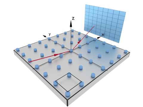
We consider a 2d Bravais lattice that is specified by lattice constants $a$ and $b$, by the angle $\alpha$ between the lattice vectors $\mathbf{a}$ and $\mathbf{b}$, and by the angle $\xi$ between $\mathbf{a}$ and the $x$ axis of the instrument frame.

The interference function for an infinite 2d lattice is created using its constructor
Interference2DLattice(length_a, length_b, alpha, xi=0)
To account for finite-size effects, and to give the simulated Bragg peaks a finite width, it is necessary to attach a peak profile (decay function), as described below.
The structure factor of the finite 2d lattice model is computed by explicit summation over contribution from all unit cells. The 2d lattice is constructed by one of the following:
BasicLattice2D(length_a, length_b, alpha, xi)
SquareLattice2D(length, xi)
HexagonalLattice2D(length, xi)
Then the interference function is constructed by
InterferenceFinite2DLattice(lattice, Na, Nb)
where the integer arguments $N_a$ and $N_b$ are the numbers of unit cells in lattice directions $\mathbf{a}$ and $\mathbf{b}$.
The decay function, which should be assigned to the interference function, accounts for the finite size of the sample or the crystalline domain or the scattering volume. It contributes a multiplicative factor $h(\mathbf{r})$ to the correlation function in real space that lets them decay for $r$. Equivalently, its Fourier transform $H(\mathbf{q})$ is convolved with the structure factor of the ideal, infinite lattice, $$S_0(\mathbf{q}) = \rho \sum_i c_i \delta(\mathbf{q} - \mathbf{q}_i),$$ where the sum runs of reciprocal lattice points, resulting in $$S(\mathbf{q}) = \rho \sum_i c_i H(\mathbf{q} - \mathbf{q}_i).$$ That is, each Bragg peak gets the same smooth profile $H(\mathbf{q})$ instead of the infinitely sharp delta function.

Decay functions for the one-dimensional case are explained in the grating section. Decay functions for two-dimensional lattices work similarly, but require two length parameters and an orientation to be defined. The lengths $\omega_x$ and $\omega_y$ refer to the principal axes of an ellipsis that is rotated by an angle $\gamma$ with respect to the coordinate axes $x$, $y$.
BornAgain supports three two-dimensional decay functions:
Profile2DCauchy(omega_x, omega_y, gamma)
Profile2DGauss(omega_x, omega_y, gamma)
Profile2DVoigt(omega_x, omega_y, gamma, eta)
The Cauchy distribution is in physics better known as the Lorentzian profile.
The Voigt distribution is computed as the true convolution
of a Gaussian and a Lorentzian, using our numeric library libcerf.
The dimensionless parameter eta=$\eta$ may take values between
0 (Lorentian) and 1 (Gaussian).
Decay lengths should be much larger than the lattice constants. Otherwise the model becomes physically questionable, and computation times increase a lot. Typical values for meaningful decay lengths are in the micrometer range (≥ 1000 nm).
The decay function is attached to an interference function by
the setDecayFunction method,
which should be called after the interference function is constructed:
iff = Interference2DLattice(20*nm, 20*nm, 120*deg)
profile = Profile2DCauchy(1000*nm, 1000*nm, 0*deg)
iff.setDecayFunction(profile)
The computational kernel provides an automatic calculation of particle densities using the parameters of the 2D lattice. This means that the user’s setting of the particle density via the ParticleLayout.setParticleDensity() method (which is a required step in the case of a 1D interference function and radial paracrystal initialization) is ignored.