A GISAS data fit deals with the following 5 components:
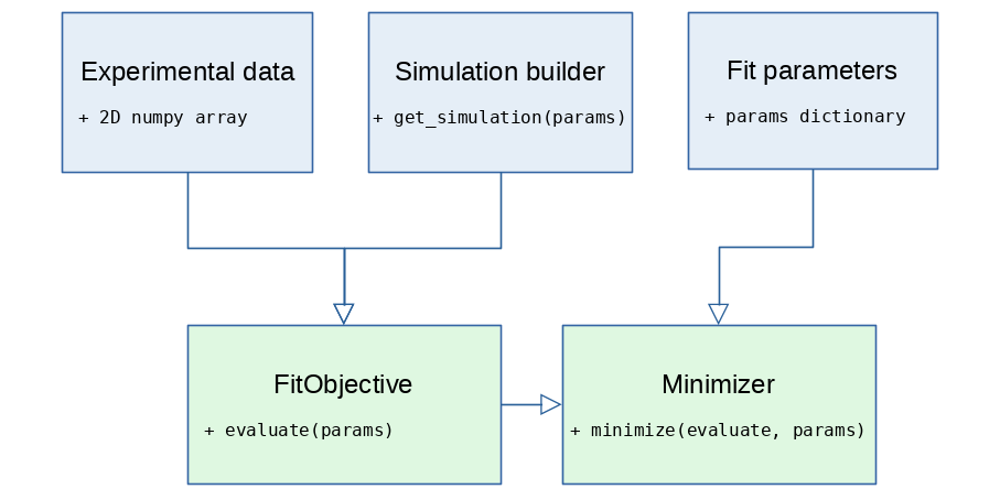
The experimental data is a 2D numpy array, obtained in the course of a GISAS experiment and containing a 2D map of the intensities measured in the detector channels.
This is a Python callable, a function or a class method, returning a ScatteringSimulation object with beam, detector and user sample defined.
The function accepts a Python dictionary as input parameters, which it uses to build a new simulation object. The parameter values will be varied during the fit and get_simulation will be called on every fit iteration.
def get_simulation(params):
    simulation = ScatteringSimulation()
    ...
    simulation.setBinIntensity(params["intensity"])
    ...
    return simulation
The main requirement here is that the geometry of the detector defined in the ScatteringSimulation object
matches the shape of numpy array with the experimental intensities.
A special module providing an objective function for the minimizer.
It contains at least one pair of experimental data/simulation builder and the logic to retrieve new simulation results on every fit iteration and compare them against the experimental one.
fit_objective = FitObjective()
fit_objective.addSimulationAndData(get_simulation, real_data)
The FitObjective public interface provides access to two objective functions
FitObjective.evaluate(params) returns $\chi_{2}$ calculated for experimental/simulated imagesFitObjective.evaluate_residuals(params) returns 1d vector of residuals for all bins of the experimental/simulated imagesA collection of fit parameters which will be varied during the fit.
The BornAgain fit parameters and minimizer interface was developed with the idea to simplify the switch between our own minimization engines and other, possibly more advanced, minimization libraries. Particularly, we have been inspired by lmfit Python package, which explains why the BornAgain setup looks very similar.
For each fit parameter one has to define a unique name, starting value and parameter bounds. The name of the fit parameter should coincide with the name that the simulation builder function expects.
params = ba.Parameters()
params.add("intensity", 1e+08, min=1e+07, max, 1e+08)
params.add("sphere_radius", 10*nm, min=0.1)
Provides the top level interface for multiple minimization engines.
In the code snippet below we create a default BornAgain minimizer and start the minimization by calling the minimize function. The minimizer takes an objective function and the fit parameters as input.
minimizer = ba.Minimizer()
minimizer.minimize(fit_objective.evaluate, params)
After all fit components are in place, the users can start the minimization by running the minimize method. The figure below shows the general workflow of a minimization procedure.
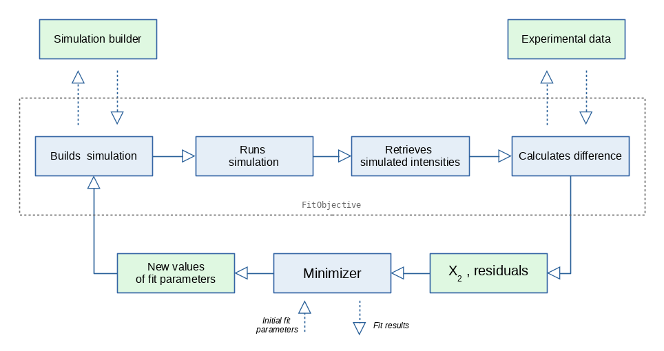
The minimization workflow involves many iterations, during each of which
The iteration process is going on under the control of the selected minimization algorithm, without any intervention from the user. It stops if one of the following is true:
After the control has returned, the fitting results can be retrieved. These include the best $\chi_{2}$ value found, the corresponding optimal sample parameter values and the intensity map simulated with this set of values.