  1
  2
  3
  4
  5
  6
  7
  8
  9
 10
 11
 12
 13
 14
 15
 16
 17
 18
 19
 20
 21
 22
 23
 24
 25
 26
 27
 28
 29
 30
 31
 32
 33
 34
 35
 36
 37
 38
 39
 40
 41
 42
 43
 44
 45
 46
 47
 48
 49
 50
 51
 52
 53
 54
 55
 56
 57
 58
 59
 60
 61
 62
 63
 64
 65
 66
 67
 68
 69
 70
 71
 72
 73
 74
 75
 76
 77
 78
 79
 80
 81
 82
 83
 84
 85
 86
 87
 88
 89
 90
 91
 92
 93
 94
 95
 96
 97
 98
 99
100
101
102
103
104
105
106
107
108
109
110
111
112
113
114
115
116
117
118
|
#!/usr/bin/env python3
"""
Extended example for simulation results treatment (cropping, slicing, exporting)
"""
import math
import random
import bornagain as ba
from bornagain import angstrom, ba_plot as bp, deg, nm, std_samples
from matplotlib import pyplot as plt
import datetime
def get_sample():
return std_samples.cylinders()
def get_simulation(sample):
"""
A GISAXS simulation with beam and detector defined.
"""
beam = ba.Beam(1e5, 1*angstrom, 0.2*deg)
n = 200
det = ba.SphericalDetector(n, -2*deg, 2*deg, n, 0, 2*deg)
simulation = ba.ScatteringSimulation(beam, sample, det)
return simulation
def get_noisy_image(field):
"""
Returns clone of input field filled with additional noise
"""
result = field.clone()
noise_factor = 2.0
for i in range(0, result.size()):
amplitude = field.valAt(i)
sigma = noise_factor*math.sqrt(amplitude)
noisy_amplitude = random.gauss(amplitude, sigma)
result.setAt(i, noisy_amplitude)
return result
def plot_histogram(field, **kwargs):
bp.plot_histogram(field,
xlabel=r'$\varphi_f ^{\circ}$',
ylabel=r'$\alpha_{\rm f} ^{\circ}$',
zlabel="",
**kwargs)
def plot_slices(noisy):
"""
Plot 1D slices along y-axis at certain x-axis values.
"""
plt.yscale('log')
# projection along Y, slice at fixed x-value
proj1 = noisy.yProjection(0)
plt.plot(proj1.axis(0).binCenters(),
proj1.flatVector(),
label=r'$\varphi=0.0^{\circ}$')
# projection along Y, slice at fixed x-value
proj2 = noisy.yProjection(0.5) # slice at fixed value
plt.plot(proj2.axis(0).binCenters(),
proj2.flatVector(),
label=r'$\varphi=0.5^{\circ}$')
# projection along Y for all X values between [xlow, xup], averaged
proj3 = noisy.yProjection(0.41, 0.59)
plt.plot(proj3.axis(0).binCenters(),
proj3.flatVector(),
label=r'$<\varphi>=0.5^{\circ}$')
plt.xlim(proj1.axis(0).min(), proj1.axis(0).max())
plt.ylim(proj1.maxVal()*3e-6, proj1.maxVal()*3)
plt.xlabel(r'$\alpha_{\rm f} ^{\circ}$', fontsize=16)
plt.legend(loc='upper right')
def plot(field):
"""
Demonstrates modified data plots.
"""
plt.subplots(2, 2, figsize=(12.80, 10.24))
plt.subplot(2, 2, 1)
bp.plot_histogram(field)
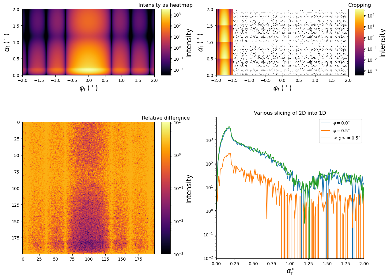
plt.title("Intensity as heatmap")
plt.subplot(2, 2, 2)
crop = field.crop(-1, 0.5, 1, 1)
bp.plot_histogram(crop)
plt.title("Cropping")
plt.subplot(2, 2, 3)
noisy = get_noisy_image(field)
reldiff = ba.relativeDifferenceField(noisy, field).npArray()
bp.plot_array(reldiff, intensity_min=1e-03, intensity_max=10)
plt.title("Relative difference")
plt.subplot(2, 2, 4)
plot_slices(noisy)
plt.title("Various slicing of 2D into 1D")
plt.tight_layout()
if __name__ == '__main__':
sample = get_sample()
simulation = get_simulation(sample)
result = simulation.simulate()
if bp.datfile:
ba.writeDatafield(result, bp.datfile + ".int.gz")
# Other supported extensions are .tif and .txt.
# Besides compression .gz, we support .bz2, and uncompressed.
field = result.extracted_field()
plot(field)
bp.show_or_export()
|