This tutorial gives a brief overview of the fitting functionality in the GUI.
As a first example, this tutorial will focus on fitting data simulated with BornAgain itself. More complex fitting examples will be addressed in coming releases. This tutorial is organized as follows:
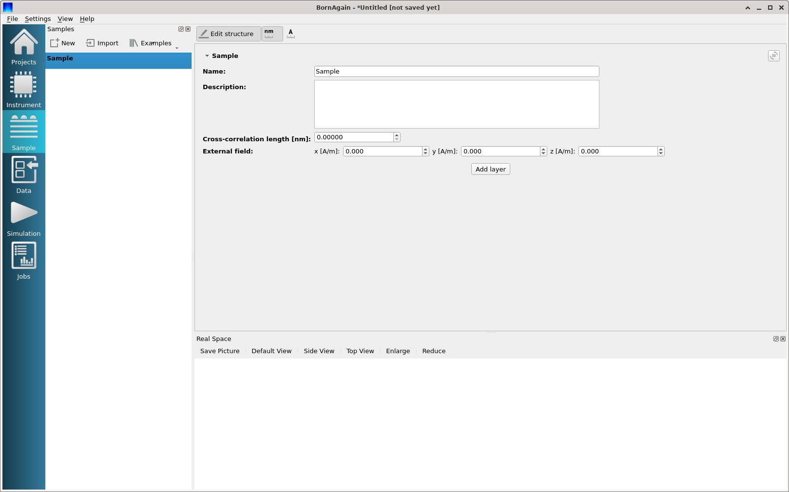
First, as explained in the GUI Overview chapter, create a project and select and instrument (here, GISAS).
Then switch to Sample View and construct a simple sample - a two-layer system (vacuum, substrate), with cylindrical particles sitting on top of the substrate. The height and radius of the cylindrical particles are both assumed to be 5 nm.
To represent the cylindrical particles in vacuum, create a new layer with the “Add layer” button.
The layer is named Layer 0.
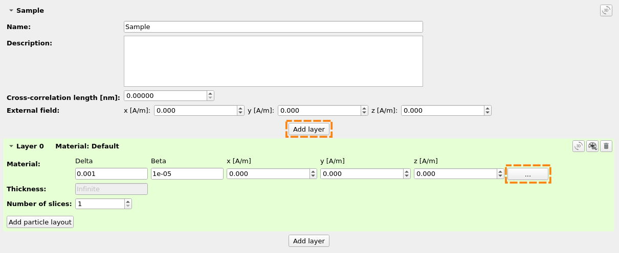
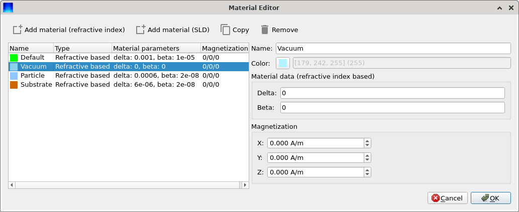
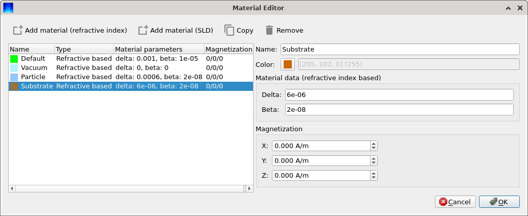
Set the layer material to “Vacuum” via the “Material Editor”, accessible via the button on the right-hand side of the layer.
To represent the cylindrical particles, create a particle layout via the “Add partice layout” button. Set the total particle density (here, 0.005/nm^2). Select the interference function (here, “None”).
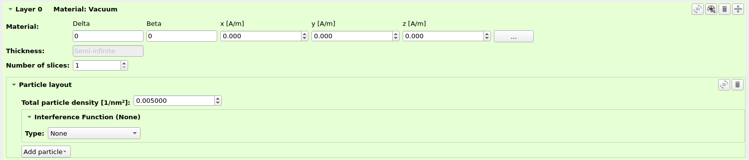
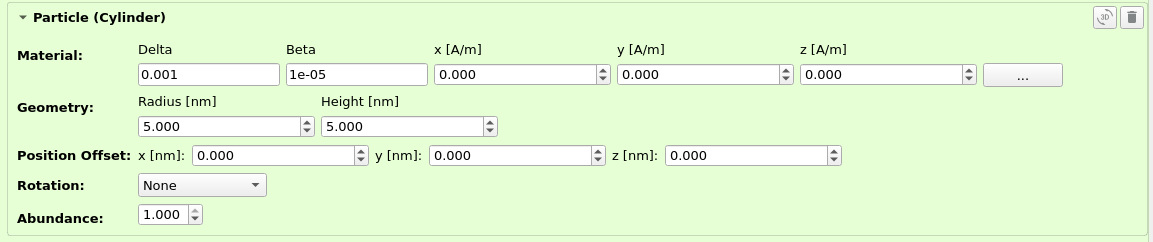
Select the particle type via the “Add particle” button (here, Hard particles->Cylinder).
Set the corresponding radius and height (here, both are 5 nm).
Add a second layer to represent the substrate (named Layer 1).
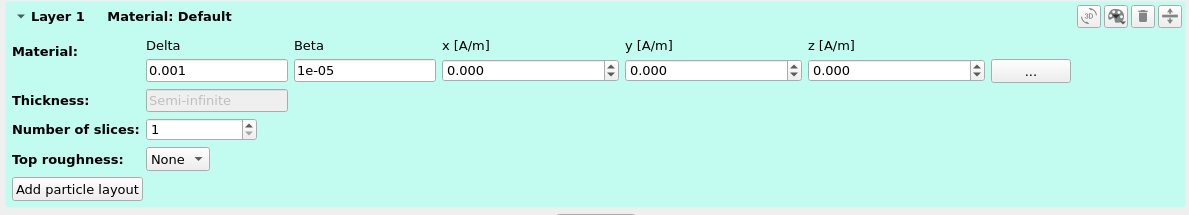
Choose the corresponding material to be “Substrate”.
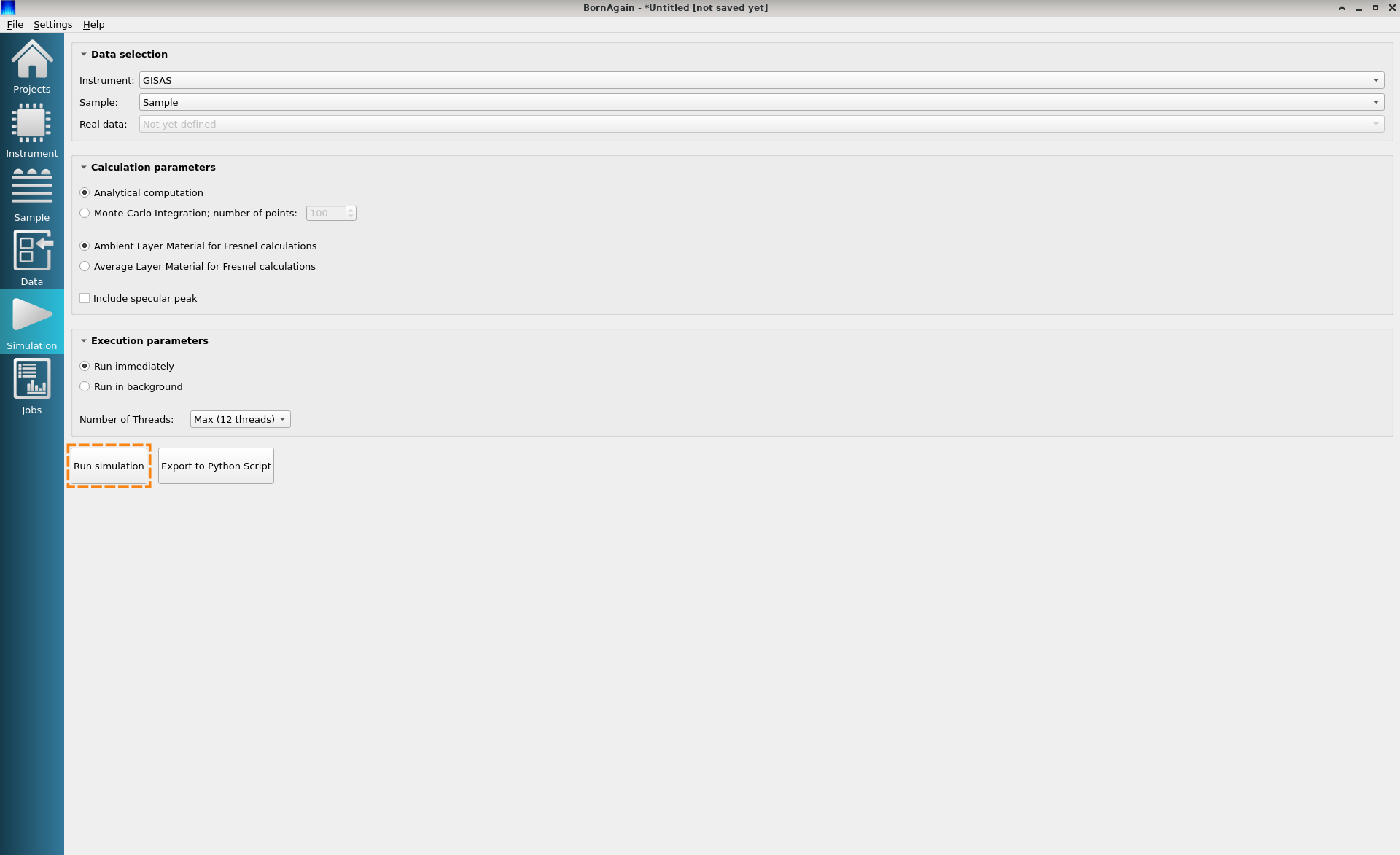
Switch to the Simulation View and run the simulation by clicking on the “Run Simulation” button.
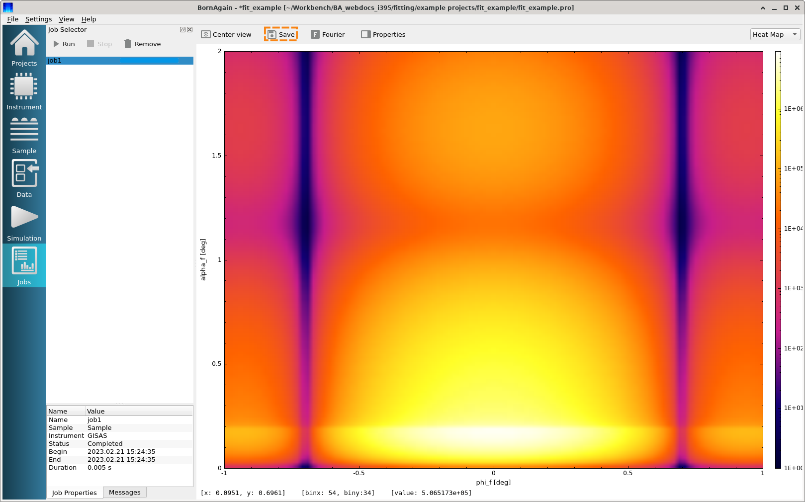
As soon as the simulation is complete, the interface automatically switches to Job View, which displays the simulated intensity map. This result can be saved as a file, in several formats; e.g., experimental_data.int in BornAgain ASCII format (*.int).
This file can be later used as an “experimental data” to be imported for fitting.
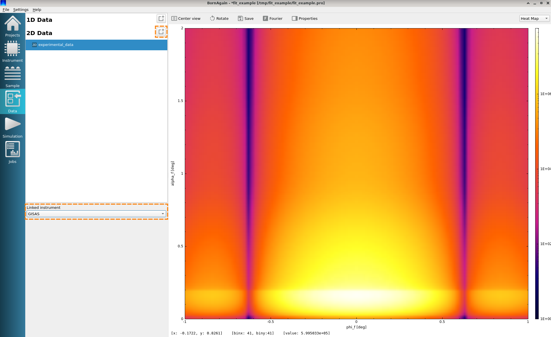
Switch to the Data View. At the beginning it is empty since there are no real data samples loaded yet. Click the import button corresponding to the 2D Data and select the experimental data file (here, experimental_data.int which was created earlier).
The data will be loaded into BornAgain and presented in the Import Data view as shown below.
Remember to set the instrument linked to the data (here, “GISAS”).
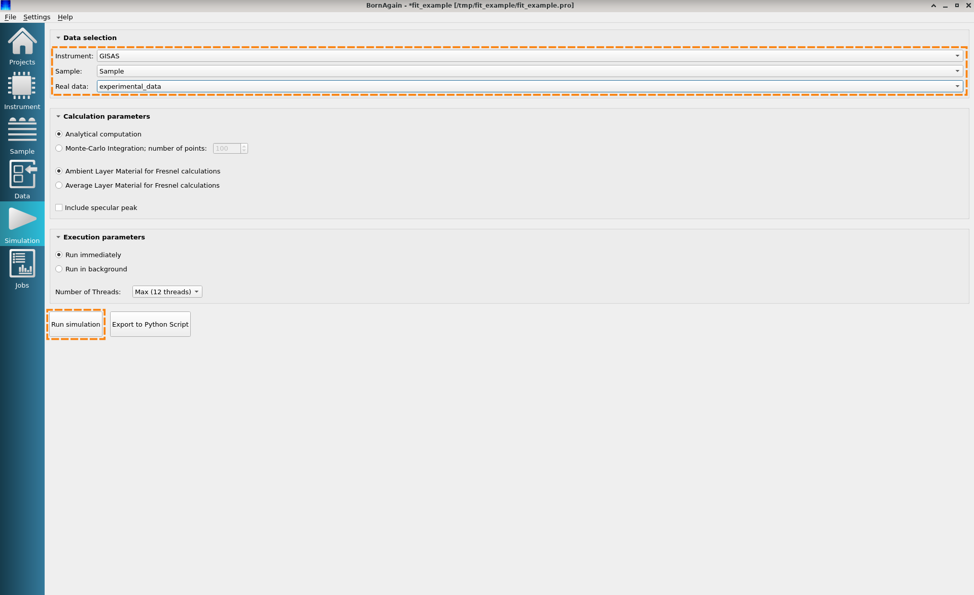
To setup the fitting job, switch back to the Simulation View. In the “Real Data” field, select the name of the real (experimental) dataset which was imported. Now, the data selection box states, as shown below, that an instrument “GISAS” will be used together with the sample “Sample”, which represents the multilayer with cylinders that was constructed in section 1, in order to fit the dataset “experimental_data”. Click on the “Run Simulation” button to start the simulation.
Once the simulation is complete, the display is once again switched to the Job View. Our current job is now ready for fitting. Switch to “Fitting Activity” via the menu View->Fitting Activity. By default, when real data has been selected in Simulation view, the current view will already be switched to the Fitting Activity.
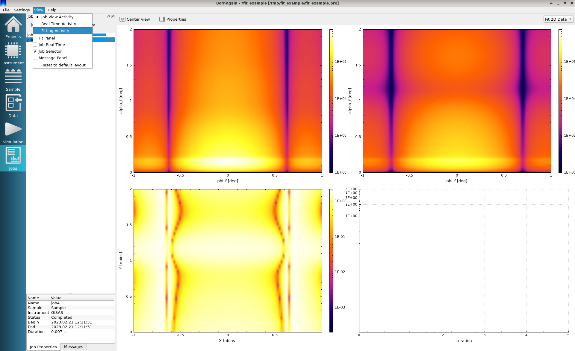
In the Fitting Activity view (below) the following elements are visible:
Furthermore, the presentation selector drop-down button allows to switch quickly between views from current “Fit Data” to standard “Heat Map”.
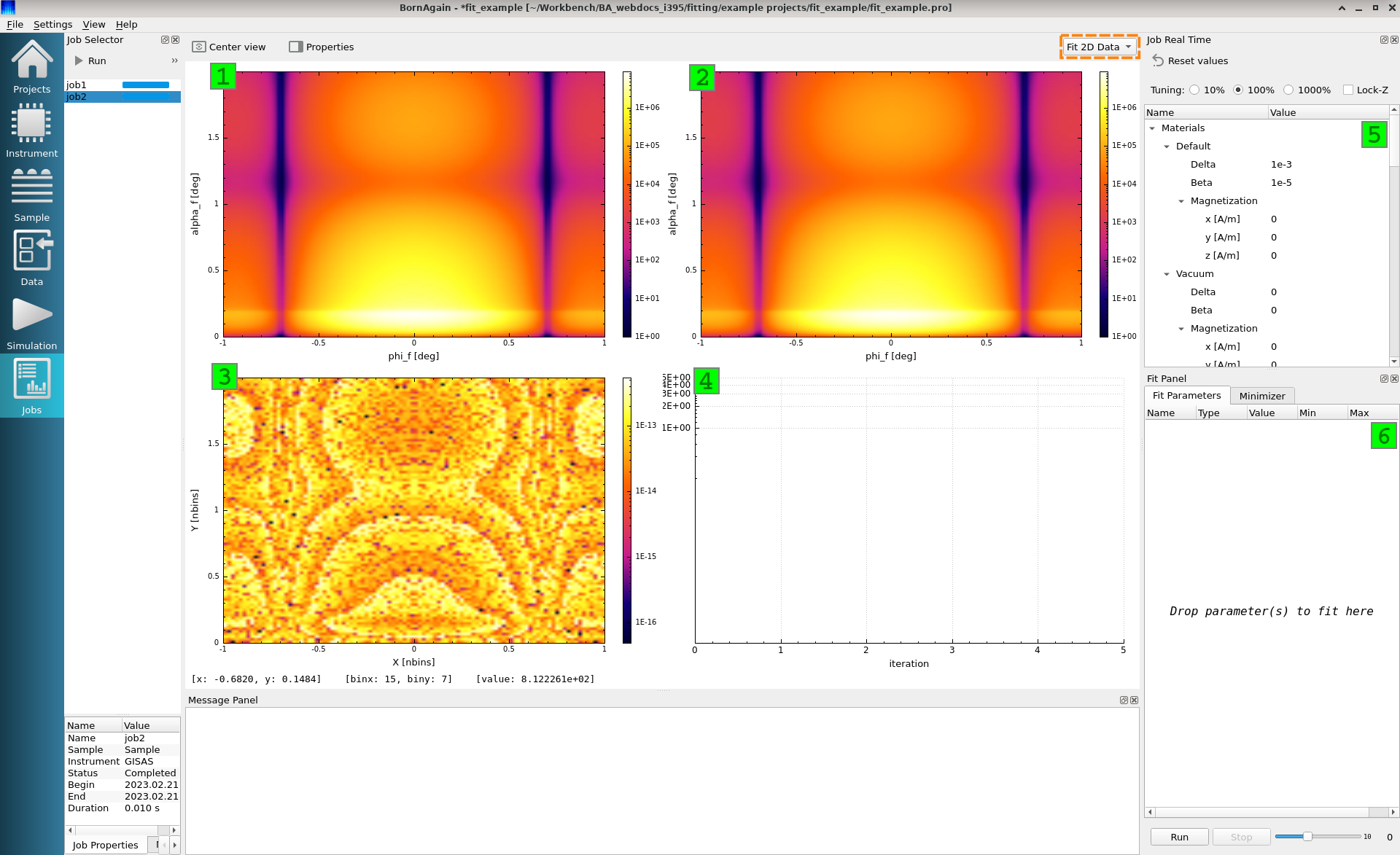
As you may see, the relative difference map (3) shows that there is actually no difference between “experimental” and “simulated” data, except for floating-point errors. This is normal, since our “experimental” data was generated using the same sample/instrument settings as the simulation. Or, in other words, at this point no fitting is required - our sample parameters perfectly describe the “experimental” data. In the following paragraph we are going to change that.
Using the parameter tuning widget on the right we set new values for two sample parameters: the cylinder radius and the cylinder height. This leads to an automatic re-simulation and update of the views: the simulated intensity map has changed and does not coincide with the “experimental” data map anymore. The relative difference map also shows this difference.
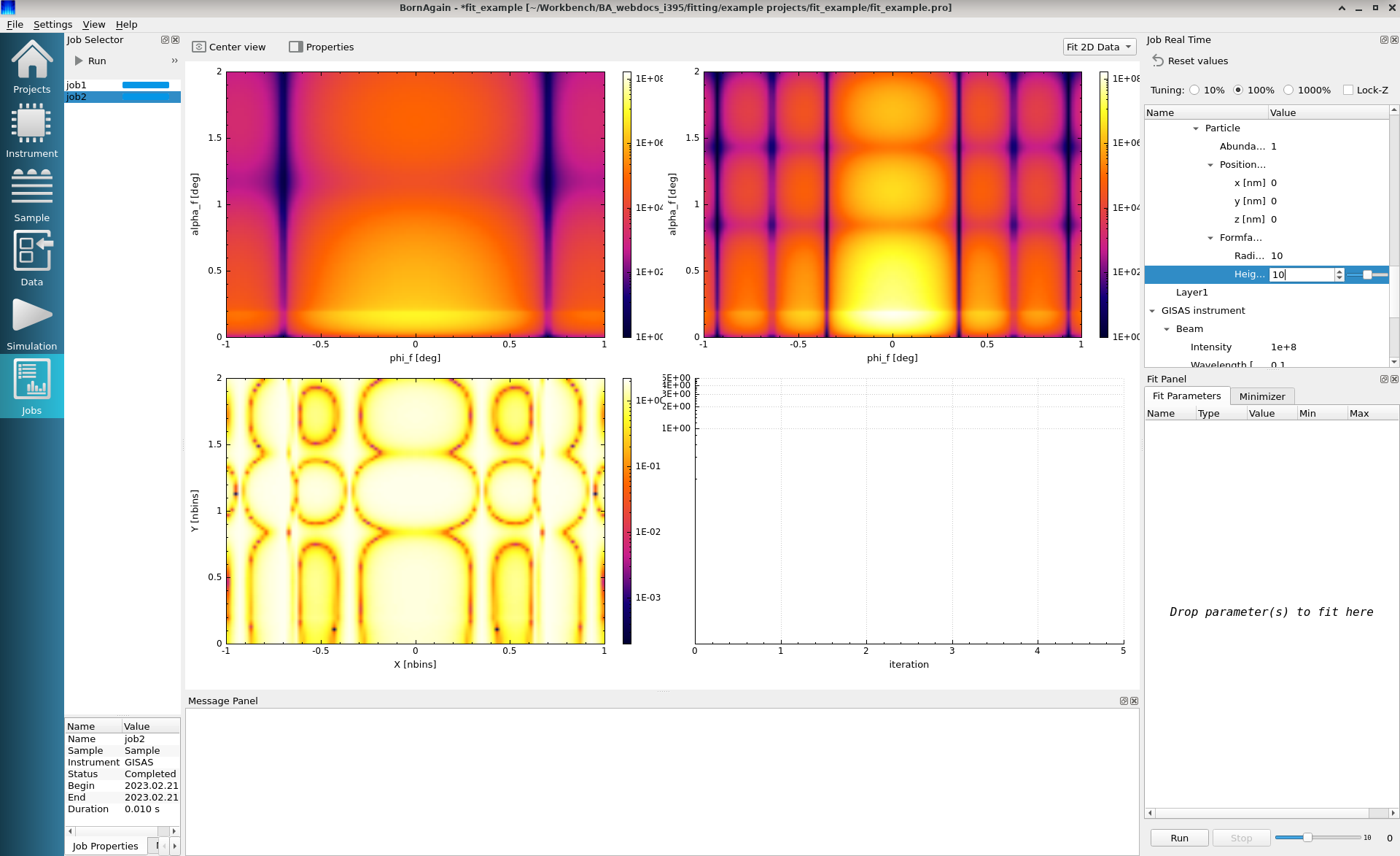
These will be the initial conditions of our fitting. The real data was simulated using values for the cylinder’s height = radius = 5 nm. The simulated intensity map is obtained for the cylinder’s height = radius = 10 nm. We are going to define two fit parameters for the cylinder’s radius and height. Our final goal is to find the original values; i.e., height = radius = 5 nm.
To create the fit parameters, drag-and-drop “radius” and “height” from the parameter tuning widget to the fit parameters widget below (indicated in the figure below).
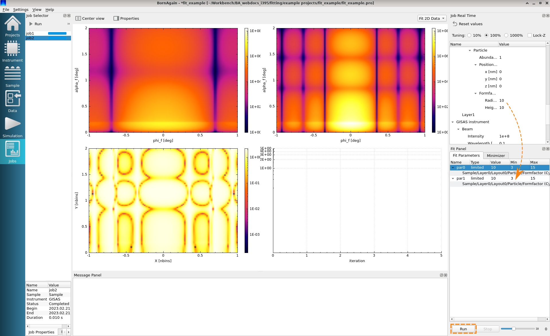
Every fit parameter has the following fields
Define the fit parameter limits: min = 3 nm, max = 15 nm and starting value = 10 nm.
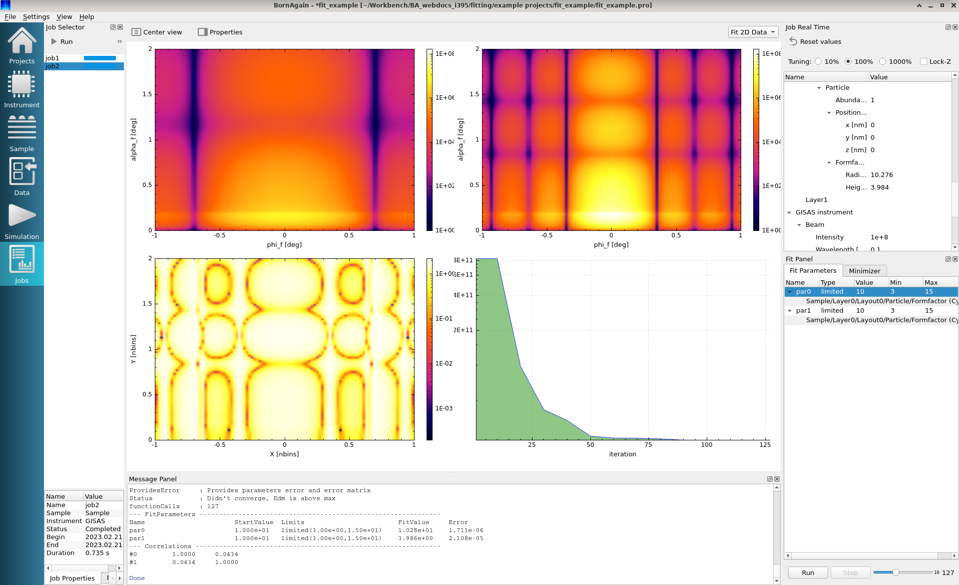
Push the “Run” button at the bottom of the “Fit Parameters” view. The fitting should start. Using the slider at the bottom area one can change the rate of updating the plot. The plot below shows the view after the fitting was completed. The green histogram in the lower right corner shows how $\chi^2$ evolves as a function of the number of fit iterations. The resulting messages are printed in the Message panel.