This example demonstrates fitting of 2D GISAS data.
The sample and instrument model is basically the same as in our basic GISAS simulation example, except that it depends on four external parameters: beam intensity, detector background, radius and height of the cylindrical nanoparticles.
Faked experimental data have been generated by the script devtools/fakeData/fake-gisas1.py .
The intensity for each detector pixel has been drawn at random from a Poisson distribution, with rate basically given by the fit model except for some imperfections that have been introduced on purpose to make the subsequent fitting more difficult and more realistic:
The faked data can be found at Examples/data/faked-gisas1.txt.gz .
The fit script shown and discussed below displays its progress visually, and terminates with the following result:
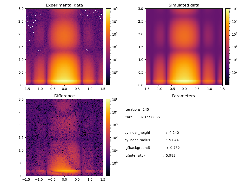
Fit window
|
|
The function get_sample is basically the same as
in our basic GISAS simulation example,
except that radius and height of the cylindrical disks are now
supplied as external parameters.
These parameters are passed through the function argument params
which can be either a Python dict,
or an instance of the BornAgain class Parameters.
The function get_simulation has the same function argument params,
from which it takes beam intensity and background level.
These two parameters are on a logarithmic scale.
The function start_parameters_1 is supplied along with the model
in order to facilitate the benchmarking of different fith methods.
The FitObjective created here is used to put into correspondence the real data,
represented by a numpy array, and the simulation, represented by the get_simulation callable.
On every fit iteration FitObjective
get_simulation callable,The method fit_objective.evaluate provided by the FitObjective class interface is used here as an objective function.
The method accepts fit parameters and returns the $\chi^2$ value,
calculated between experimental and simulated images for the given values of the fit parameters.
The method is passed to the minimizer together with the initial fit parameter values.
The minimizer.minimize starts a fit that will
continue further without user intervention until the minimum
is found or the minimizer failed to converge.
The rest of the code demonstrates how to access the fit results.