  1
  2
  3
  4
  5
  6
  7
  8
  9
 10
 11
 12
 13
 14
 15
 16
 17
 18
 19
 20
 21
 22
 23
 24
 25
 26
 27
 28
 29
 30
 31
 32
 33
 34
 35
 36
 37
 38
 39
 40
 41
 42
 43
 44
 45
 46
 47
 48
 49
 50
 51
 52
 53
 54
 55
 56
 57
 58
 59
 60
 61
 62
 63
 64
 65
 66
 67
 68
 69
 70
 71
 72
 73
 74
 75
 76
 77
 78
 79
 80
 81
 82
 83
 84
 85
 86
 87
 88
 89
 90
 91
 92
 93
 94
 95
 96
 97
 98
 99
100
101
102
103
104
105
106
107
108
109
110
111
112
113
114
115
116
117
118
119
120
121
122
123
124
125
126
127
128
129
130
131
|
#!/usr/bin/env python3
"""
Extended example for simulation results treatment (cropping, slicing, exporting)
"""
import math
import random
import bornagain as ba
from bornagain import angstrom, ba_plot as bp, deg, nm, std_samples
from matplotlib import pyplot as plt
def get_sample():
return std_samples.cylinders()
def get_simulation(sample):
"""
Returns a GISAXS simulation with beam and detector defined.
"""
beam = ba.Beam(1e5, 1*angstrom, 0.2*deg)
n = bp.simargs['n']
det = ba.SphericalDetector(n, -2*deg, 2*deg, n, 0, 2*deg)
simulation = ba.ScatteringSimulation(beam, sample, det)
return simulation
def get_noisy_image(field):
"""
Returns clone of input field filled with additional noise
"""
result = field.clone()
noise_factor = 2.0
for i in range(0, result.size()):
amplitude = field.valAt(i)
sigma = noise_factor*math.sqrt(amplitude)
noisy_amplitude = random.gauss(amplitude, sigma)
result.setAt(i, noisy_amplitude)
return result
def plot_histogram(field, **kwargs):
bp.plot_histogram(field,
xlabel=r'$\varphi_f ^{\circ}$',
ylabel=r'$\alpha_{\rm f} ^{\circ}$',
zlabel="",
**kwargs)
def plot_slices(field):
"""
Plot 1D slices along y-axis at certain x-axis values.
"""
noisy = get_noisy_image(field)
plt.yscale('log')
# projection along Y, slice at fixed x-value
proj1 = noisy.yProjection(0)
plt.plot(proj1.axis(0).binCenters(),
proj1.flatVector(),
label=r'$\varphi=0.0^{\circ}$')
# projection along Y, slice at fixed x-value
proj2 = noisy.yProjection(0.5) # slice at fixed value
plt.plot(proj2.axis(0).binCenters(),
proj2.flatVector(),
label=r'$\varphi=0.5^{\circ}$')
# projection along Y for all X values between [xlow, xup], averaged
proj3 = noisy.yProjection(0.41, 0.59)
plt.plot(proj3.axis(0).binCenters(),
proj3.flatVector(),
label=r'$<\varphi>=0.5^{\circ}$')
plt.xlim(proj1.axis(0).min(), proj1.axis(0).max())
plt.ylim(proj2.minVal(), proj1.maxVal()*10)
plt.xlabel(r'$\alpha_{\rm f} ^{\circ}$', fontsize=16)
plt.legend(loc='upper right')
plt.tight_layout()
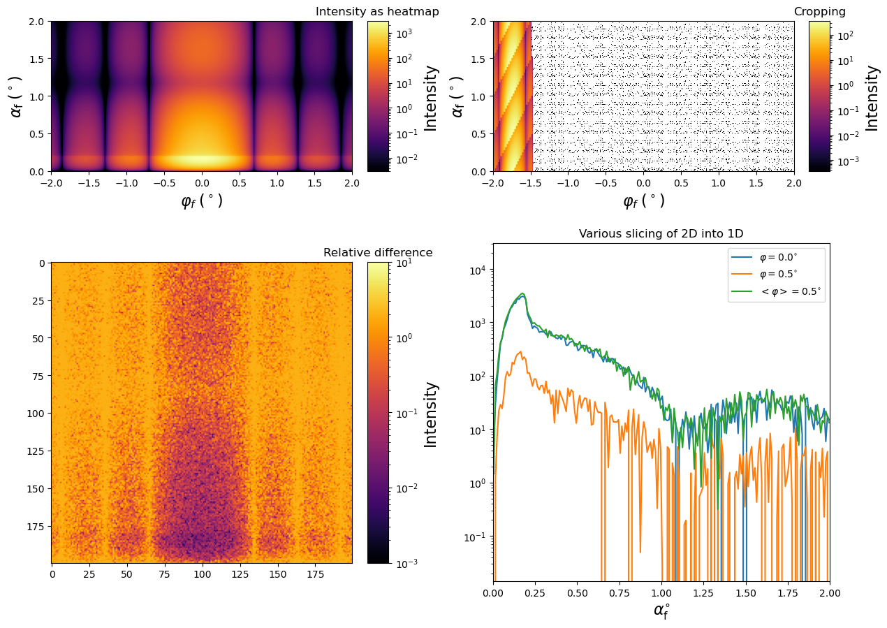
def plot(field):
"""
Demonstrates modified data plots.
"""
plt.figure(figsize=(12.80, 10.24))
print("Subplot 1")
plt.subplot(2, 2, 1)
bp.plot_histogram(field)
plt.title("Intensity as heatmap")
print("Subplot 2")
plt.subplot(2, 2, 2)
crop = field.crop(-1, 0.5, 1, 1)
bp.plot_histogram(crop)
plt.title("Cropping")
print("Subplot 3")
plt.subplot(2, 2, 3)
noisy = get_noisy_image(field)
reldiff = ba.relativeDifferenceField(noisy, field).npArray()
bp.plot_array(reldiff, intensity_min=1e-03, intensity_max=10)
plt.title("Relative difference")
print("Subplot 4")
plt.subplot(2, 2, 4)
plot_slices(field)
plt.title("Various slicing of 2D into 1D")
print("Layout")
plt.tight_layout()
if __name__ == '__main__':
bp.parse_args(sim_n=200)
sample = get_sample()
simulation = get_simulation(sample)
print("Simulate")
result = simulation.simulate()
if bp.datfile:
print("Save results")
ba.IOFactory.writeSimulationResult(result, bp.datfile + ".int.gz")
# Other supported extensions are .tif and .txt.
# Besides compression .gz, we support .bz2, and uncompressed.
print("Get datafield")
field = result.datafield()
print("Plot")
plot(field)
bp.show_or_export()
|