  1
  2
  3
  4
  5
  6
  7
  8
  9
 10
 11
 12
 13
 14
 15
 16
 17
 18
 19
 20
 21
 22
 23
 24
 25
 26
 27
 28
 29
 30
 31
 32
 33
 34
 35
 36
 37
 38
 39
 40
 41
 42
 43
 44
 45
 46
 47
 48
 49
 50
 51
 52
 53
 54
 55
 56
 57
 58
 59
 60
 61
 62
 63
 64
 65
 66
 67
 68
 69
 70
 71
 72
 73
 74
 75
 76
 77
 78
 79
 80
 81
 82
 83
 84
 85
 86
 87
 88
 89
 90
 91
 92
 93
 94
 95
 96
 97
 98
 99
100
101
102
103
104
105
106
107
108
109
110
111
112
113
114
115
116
117
118
119
120
121
122
123
124
125
126
127
128
129
130
131
132
133
134
135
136
137
138
139
140
141
142
143
144
145
146
147
148
149
150
151
152
153
154
155
156
157
158
159
160
161
162
163
164
165
166
167
168
169
170
171
172
173
174
175
176
177
178
179
180
181
182
183
184
185
186
187
188
189
190
191
192
193
194
195
196
197
198
199
200
201
202
203
204
205
206
207
208
209
210
211
212
213
214
215
216
217
218
219
220
221
222
223
224
225
226
227
228
229
230
231
232
233
234
235
236
237
238
239
240
241
242
243
244
245
|
#!/usr/bin/env python3
"""
This simulation example demonstrates how to replicate the
fitting example "Magnetically Dead Layers in Spinel Films"
given at the Nist website:
https://www.nist.gov/ncnr/magnetically-dead-layers-spinel-films
For simplicity, here we only reproduce the first part of that
demonstration without the magnetically dead layer.
"""
import os
import numpy
import matplotlib.pyplot as plt
import bornagain as ba
from bornagain import angstrom, ba_plot as bp, deg, R3
# q-range on which the simulation and fitting are to be performed
qmin = 0.05997
qmax = 1.96
# number of points on which the computed result is plotted
scan_size = 1500
# The SLD of the substrate is kept constant
sldMao = (5.377e-06, 0)
# constant to convert between magnetization and magnetic SLD
RhoMconst = 2.910429812376859e-12
####################################################################
# Create Sample and Simulation #
####################################################################
def get_sample(params):
"""
construct the sample with the given parameters
"""
magnetizationMagnitude = params["rhoM_Mafo"]*1e-6/RhoMconst
angle = 0
magnetizationVector = R3(
magnetizationMagnitude*numpy.sin(angle*deg),
magnetizationMagnitude*numpy.cos(angle*deg), 0)
mat_vacuum = ba.MaterialBySLD("Vacuum", 0, 0)
mat_layer = ba.MaterialBySLD("(Mg,Al,Fe)3O4", params["rho_Mafo"]*1e-6,
0, magnetizationVector)
mat_substrate = ba.MaterialBySLD("MgAl2O4", *sldMao)
ambient_layer = ba.Layer(mat_vacuum)
layer = ba.Layer(mat_layer, params["t_Mafo"]*angstrom)
substrate_layer = ba.Layer(mat_substrate)
r_Mafo = ba.LayerRoughness(params["r_Mafo"]*angstrom)
r_substrate = ba.LayerRoughness(params["r_Mao"]*angstrom)
sample = ba.MultiLayer()
sample.addLayer(ambient_layer)
sample.addLayerWithTopRoughness(layer, r_Mafo)
sample.addLayerWithTopRoughness(substrate_layer, r_substrate)
return sample
def get_simulation(sample, q_axis, parameters, polarizer_dir,
analyzer_dir):
"""
Returns a simulation object.
Polarization, analyzer and resolution are set
from given parameters
"""
q_axis = q_axis + parameters["q_offset"]
distr = ba.DistributionGaussian(0., 1., 25, 4.)
scan = ba.QzScan(q_axis)
scan.setAbsoluteQResolution(distr, parameters["q_res"])
# TODO CHECK not parameters["q_res"]*q_axis ??
scan.setPolarization(polarizer_dir)
scan.setAnalyzer(analyzer_dir, 1, 0.5)
return ba.SpecularSimulation(scan, sample)
def run_simulation(q_axis, fitParams, *, polarizer_dir, analyzer_dir):
"""
Run a simulation on the given q-axis, where the sample is
constructed with the given parameters.
Vectors for polarization and analyzer need to be provided
"""
parameters = dict(fitParams, **fixedParams)
sample = get_sample(parameters)
simulation = get_simulation(sample, q_axis, parameters, polarizer_dir,
analyzer_dir)
return simulation.simulate()
def qr(result):
"""
Returns two arrays that hold the q-values as well as the
reflectivity from a given simulation result
"""
q = numpy.array(result.convertedBinCenters(ba.Coords_QSPACE))
r = numpy.array(result.array(ba.Coords_QSPACE))
return q, r
####################################################################
# Plot Handling #
####################################################################
def plot(qs, rs, exps, labels, filename):
"""
Plot the simulated result together with the experimental data
"""
fig = plt.figure()
ax = fig.add_subplot(111)
for q, r, exp, l in zip(qs, rs, exps, labels):
ax.errorbar(exp[0],
exp[1],
xerr=exp[3],
yerr=exp[2],
fmt='.',
markersize=0.75,
linewidth=0.5)
ax.plot(q, r, label=l)
ax.set_yscale('log')
plt.legend()
plt.xlabel("Q [nm${}^{-1}$]")
plt.ylabel("R")
plt.tight_layout()
plt.savefig(filename)
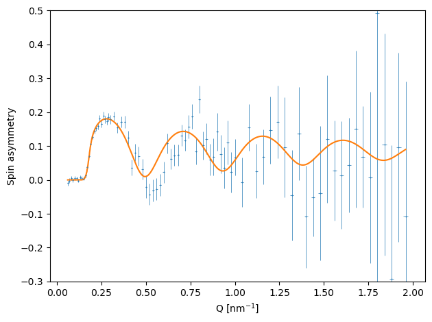
def plotSpinAsymmetry(data_pp, data_mm, q, r_pp, r_mm, filename):
"""
Plot the simulated spin asymmetry as well its
experimental counterpart with errorbars
"""
# compute the errorbars of the spin asymmetry
delta = numpy.sqrt(4 * (data_pp[1]**2 * data_mm[2]**2 + \
data_mm[1]**2 * data_pp[2]**2 ) /
( data_pp[1] + data_mm[1] )**4 )
fig = plt.figure()
ax = fig.add_subplot(111)
ax.errorbar(data_pp[0],
(data_pp[1] - data_mm[1])/(data_pp[1] + data_mm[1]),
xerr=data_pp[3],
yerr=delta,
fmt='.',
markersize=0.75,
linewidth=0.5)
ax.plot(q, (r_pp - r_mm)/(r_pp + r_mm))
plt.gca().set_ylim((-0.3, 0.5))
plt.xlabel("Q [nm${}^{-1}$]")
plt.ylabel("Spin asymmetry")
plt.tight_layout()
plt.savefig(filename)
####################################################################
# Data Handling #
####################################################################
def load_exp(fname):
dat = numpy.loadtxt(fname)
return numpy.transpose(dat)
def filterData(data, qmin, qmax):
minIndex = numpy.argmin(numpy.abs(data[0] - qmin))
maxIndex = numpy.argmin(numpy.abs(data[0] - qmax))
return data[:, minIndex:maxIndex + 1]
####################################################################
# Main Function #
####################################################################
if __name__ == '__main__':
bp.parse_args()
datadir = os.getenv('BA_EXAMPLE_DATA_DIR', '')
fname_stem = os.path.join(datadir, "MAFO_Saturated_")
expdata_pp = load_exp(fname_stem + "pp.tab")
expdata_mm = load_exp(fname_stem + "mm.tab")
fixedParams = {
# parameters from our own fit run
'q_res': 0.010542945012551425,
'q_offset': 7.971243487467318e-05,
'rho_Mafo': 6.370140108715461,
'rhoM_Mafo': 0.27399566816062926,
't_Mafo': 137.46913056084736,
'r_Mao': 8.60487712674644,
'r_Mafo': 3.7844265311293483
}
def run_Simulation_pp(qzs, params):
return run_simulation(qzs,
params,
polarizer_dir=R3(0, 1, 0),
analyzer_dir=R3(0, 1, 0))
def run_Simulation_mm(qzs, params):
return run_simulation(qzs,
params,
polarizer_dir=R3(0, -1, 0),
analyzer_dir=R3(0, -1, 0))
qzs = numpy.linspace(qmin, qmax, scan_size)
q_pp, r_pp = qr(run_Simulation_pp(qzs, fixedParams))
q_mm, r_mm = qr(run_Simulation_mm(qzs, fixedParams))
data_pp = filterData(expdata_pp, qmin, qmax)
data_mm = filterData(expdata_mm, qmin, qmax)
plot([q_pp, q_mm], [r_pp, r_mm], [data_pp, data_mm], ["$++$", "$--$"],
"MAFO_Saturated.pdf")
plotSpinAsymmetry(data_pp, data_mm, qzs, r_pp, r_mm,
"MAFO_Saturated_spin_asymmetry.pdf")
bp.show_or_export()
|