Size-distribution models

Local monodisperse approximation

The LMA approach implies that the layer is laterally divided into domains containing particles of the same size and shape and organized into a certain structure. In this approximation the domains are spatially separated and thus completely independent from each other.

The scattering intensity is incoherently summed over the domains with the corresponding weights.

# Interference functions    
iff_1 = ba.InterferenceRadialParacrystal(...)
iff_2 = ba.Interference2DParacrystal(...)
...

# Structured particle layouts
layout_1 = ba.StructuredLayout(iff_1)
layout_2 = ba.StructuredLayout(iff_2)
...
layout_1.addParticle(particle_1)
layout_2.addParticle(particle_2)
...

# Populate layer with structured layouts
layer.addStruct(layout_1)
layer.addStruct(layout_2)
...
layer.depositParticle(...) # and unstructured

Decoupling approximation

The DA approach implies that the particles share the common interference function but present there with their individual weights. There is still no coherence between different types of particles.

Can be considered as a subcase of LMA.

Ordered

layout = ba.StructuredLayout(iff)
layout.addParticle(particle_1, weight_1)
layout.addParticle(particle_2, weight_2)
...
layer.addStruct(layout)

or disordered case

layer.depositParticle(density_1, particle_1)
layer.depositParticle(density_2, particle_2)
...

Size space coupling approximation

Applicable only to radial paracrystal.

The SSCA approach introduces phase shift between different fractions with the common interference function within the layout. This is done by setting parameter kappa to 1 (it is 0 by default).

iff.setKappa(1)

layout = ba.StructuredLayout(iff)
layout.addParticle(particle_1, weight_1)
layout.addParticle(particle_2, weight_2)
...
layer.addStruct(layout)

Example

Scattering from a distribution of cylinders of two different sizess, positioned according to the radial paracrystal model.

  • The sample is made of cylinders deposited on a substrate.

  • The distribution of particles is made of:

    • 80% of cylinders with radii and heights equal to $5$ nm
    • 20% of cylinders with radii and heights equal to $8$ nm.
  • The interference function is radial paracrystal with a peak distance of $18$ nm and a damping length of $1$ $\mu$m. (LMA: two radial paracrystals with a peak distances of $16.8$ and $22.8$ nm.)

  • The wavelength is equal to 0.1 nm.

  • The incident angles are $\alpha_i = 0.2 ^{\circ}$ and $\varphi_i = 0^{\circ}$.

The example below compares the scattering patterns of all three approximations.

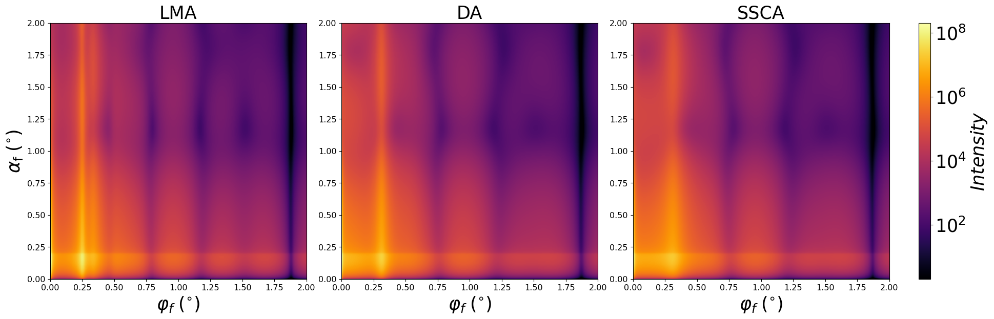
Scattering intensity

  1
  2
  3
  4
  5
  6
  7
  8
  9
 10
 11
 12
 13
 14
 15
 16
 17
 18
 19
 20
 21
 22
 23
 24
 25
 26
 27
 28
 29
 30
 31
 32
 33
 34
 35
 36
 37
 38
 39
 40
 41
 42
 43
 44
 45
 46
 47
 48
 49
 50
 51
 52
 53
 54
 55
 56
 57
 58
 59
 60
 61
 62
 63
 64
 65
 66
 67
 68
 69
 70
 71
 72
 73
 74
 75
 76
 77
 78
 79
 80
 81
 82
 83
 84
 85
 86
 87
 88
 89
 90
 91
 92
 93
 94
 95
 96
 97
 98
 99
100
101
102
103
104
105
106
107
108
109
110
111
112
113
114
#!/usr/bin/env python3
"""
Cylinders of two different sizes in Decoupling Approximation,
Local Monodisperse Approximation and Size-Spacing Coupling Approximation
"""
import bornagain as ba
from bornagain import ba_plot as bp, deg, nm


def get_sample(approximation):
    """
    A sample with cylinders of two different sizes on a substrate
    in radial paracrystal ordering.
    """

    # Materials
    material_particle = ba.RefractiveMaterial("Particle", 0.0006, 2e-08)
    material_substrate = ba.RefractiveMaterial("Substrate", 6e-06, 2e-08)
    vacuum = ba.RefractiveMaterial("Vacuum", 0, 0)

    # Particles
    ff_1 = ba.Cylinder(5*nm, 5*nm)
    ff_2 = ba.Cylinder(8*nm, 8*nm)
    particle_1 = ba.Particle(material_particle, ff_1)
    particle_2 = ba.Particle(material_particle, ff_2)

    # Layers
    layer_1 = ba.Layer(vacuum)
    layer_2 = ba.Layer(material_substrate)
    
    # Distribution function
    profile = ba.Profile1DGauss(3*nm)
    
    if (not approximation=='LMA' and
        not approximation=='DA' and
        not approximation=='SSCA'):
        raise Exception('Unknown approximation')
         
    if approximation == 'LMA':
        """
        Local Monodisperse Approximation: two independent layouts
        with their own distinct interference functions
        """
        # Interference functions
        iff_1 = ba.InterferenceRadialParacrystal(16.8*nm, 1000*nm)
        iff_2 = ba.InterferenceRadialParacrystal(22.8*nm, 1000*nm)
        iff_1.setProbabilityDistribution(profile)
        iff_2.setProbabilityDistribution(profile)

        # Particle layouts
        layout_1 = ba.StructuredLayout(iff_1)
        layout_1.addParticle(particle_1, 0.8)
        layout_2 = ba.StructuredLayout(iff_2)
        layout_2.addParticle(particle_2, 0.2)
        
        # Populate layer with two independent layouts
        layer_1.addStruct(0.5, layout_1)
        layer_1.addStruct(0.5, layout_2)
        
    else: # 'DA/SSCA'
        iff = ba.InterferenceRadialParacrystal(18*nm, 1000*nm)
        profile = ba.Profile1DGauss(3*nm)
        iff.setProbabilityDistribution(profile)
        
        """
        The only difference between Decoupling Approximation and
        Size-Spacing Coupling Approximation is that in SSCA there is
        a position phase offset between fractions defined by 'kappa' parameter:
        DA: kappa = 0 (default value)
        SSCA: kappa = 1
        """
        if approximation == 'SSCA':
            iff.setKappa(1)

        # Particle layout
        layout = ba.StructuredLayout(iff)
        layout.addParticle(particle_1, 0.8)
        layout.addParticle(particle_2, 0.2)

        # Populate layer with the layout
        layer_1.addStruct(layout)

    # Sample
    sample = ba.Sample()
    sample.addLayer(layer_1)
    sample.addLayer(layer_2)

    return sample


def get_simulation(sample):
    beam = ba.Beam(1e9, 0.1*nm, 0.2*deg)
    n = 200
    detector = ba.SphericalDetector(n, 0., 2*deg, n, 0., 2*deg)
    simulation = ba.ScatteringSimulation(beam, sample, detector)
    return simulation


def simulate(approximation):
    sample = get_sample(approximation)
    simulation = get_simulation(sample)
    result = simulation.simulate()
    result.setTitle(approximation)
    return result


if __name__ == '__main__':
    results = [
        simulate('LMA'), 
        simulate('DA'), 
        simulate('SSCA')
    ]
    bp.plot_to_row(results)
    bp.plt.show()
auto/Examples/scatter2d/Approximations.py