 BornAgain
≻ git-develop
≻ Documentation ≻ Reference ≻ Sample model ≻ Particles ≻ Form factor ≻ Custom formfactor
BornAgain
≻ git-develop
≻ Documentation ≻ Reference ≻ Sample model ≻ Particles ≻ Form factor ≻ Custom formfactor
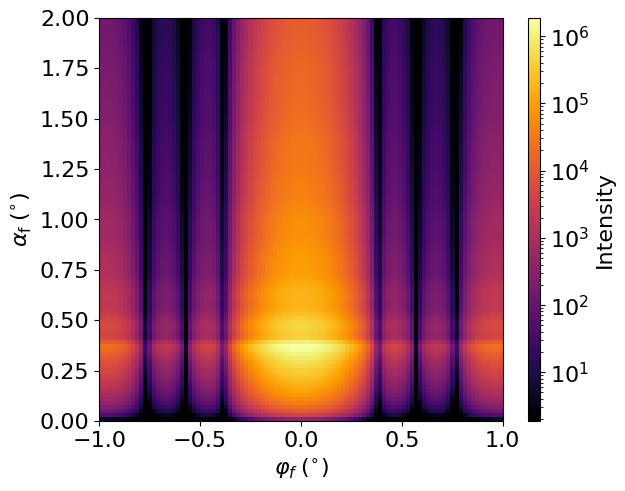
Scattering from a monodisperse distribution of particles, whose form factor is defined by the user.
The form-factor function receives a C3 vector q with
complex components in nm⁻¹. Read them with q.x(), q.y(), and q.z().
For the expression qx*qx + qy*qy + qz*qz, use q.analytic_square().
q.mag2() instead sums absolute squares and gives a different result for
complex components:
import bornagain as ba

q = ba.C3(1 + 1j, 0, 0)
q.analytic_square()  # 2j
q.mag2()             # 2.0
Use q.analytic_square_xy() for qx*qx + qy*qy. These expressions preserve
the analytic form of formulas evaluated at complex momentum transfer.

Real-space model
Scattering intensity