1
  2
  3
  4
  5
  6
  7
  8
  9
 10
 11
 12
 13
 14
 15
 16
 17
 18
 19
 20
 21
 22
 23
 24
 25
 26
 27
 28
 29
 30
 31
 32
 33
 34
 35
 36
 37
 38
 39
 40
 41
 42
 43
 44
 45
 46
 47
 48
 49
 50
 51
 52
 53
 54
 55
 56
 57
 58
 59
 60
 61
 62
 63
 64
 65
 66
 67
 68
 69
 70
 71
 72
 73
 74
 75
 76
 77
 78
 79
 80
 81
 82
 83
 84
 85
 86
 87
 88
 89
 90
 91
 92
 93
 94
 95
 96
 97
 98
 99
100
101
102
103
104
105
106
107
108
109
110
111
112
113
114
115
116
117
118
119
120
121
122
123
124
125
126
127
128
129
130
131
132
133
134
135
136
137
138
139
140
141
142
143
144
145
146
147
148
149
150
151
152
153
154
155
156
157
158
159
160
161
162
163
164
165
166
167
168
169
170
171
172
173
174
175
176
177
178
179
180
181
182
183
184
185
186
187
188
189
190
191
192
193
194
195
196
197
198
199
200
201
202
203
204
205
206
207
208
209
210
211
212
213
214
215
216
217
218
219
220
221
222
223
224
225
226
227
228
229
230
231
232
233
234
235
236
237
238
239
240
241
242
243
244
245
246
247
248
249
250
251
252
253
254
255
256
257
258
259
260
261
262
263
264
265
266
267
268
269
270
271
272
273
274
275
276
277
278
279
280
281
282
283
284
285
286
287
288
289
290
291
292
293
294
295
296
297
298
299
300
301
302
303
304
305
306
307
308
309
310
311
312
313
|
#!/usr/bin/env python3
# /// script
# requires-python = ">=3.10"
# dependencies = ["bornagain>=25,<26", "lmfit"]
# ///
"""
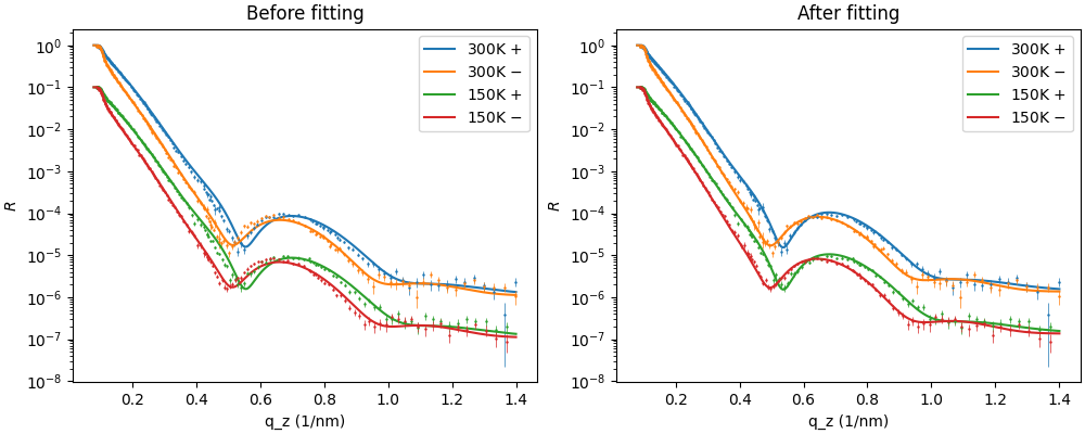
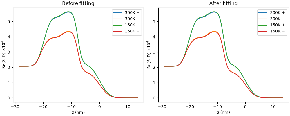
This example demonstrates how to fit a complex experimental setup using BornAgain.
It is based on real data published in  https://doi.org/10.1002/advs.201700856
by A. Glavic et al.
In this example we utilize the scalar reflectometry engine to fit polarized
data without spin-flip for performance reasons.
"""

from itertools import count
import os
from pathlib import Path

import bornagain as ba
ba.require_versions("bornagain>=25,<26")
import lmfit
import numpy as np
from bornagain import nm


####################################################################
#  Sample and simulation model
####################################################################

def get_sample(P, spin_sign, temperature):

    if temperature < 200:
        ms150 = P["ms150"]
    else:
        ms150 = 1

    air_color = (0.90, 0.93, 0.97)
    air_mat = ba.SLDMaterial("Air", air_color, 0, 0)

    pyox_color = (0.62, 0.68, 0.72)
    pyox_sld_real = (P["sld_PyOx_real"] + spin_sign*ms150*P["msld_PyOx"])*1e-6
    pyox_mat = ba.SLDMaterial("PyOx", pyox_color, pyox_sld_real, 0)

    py2_color = (0.58, 0.40, 0.74)
    py2_sld_real = (P["sld_Py2_real"] + spin_sign*ms150*P["msld_Py2"])*1e-6
    py2_mat = ba.SLDMaterial("Py2", py2_color, py2_sld_real, 0)

    py1_color = (0.05, 0.62, 0.55)
    py1_sld_real = (P["sld_Py1_real"] + spin_sign*ms150*P["msld_Py1"])*1e-6
    py1_mat = ba.SLDMaterial("Py1", py1_color, py1_sld_real, 0)

    sio2_color = (0.25, 0.74, 0.42)
    sio2_sld_real = P["sld_SiO2_real"]*1e-6
    sio2_mat = ba.SLDMaterial("SiO2", sio2_color, sio2_sld_real, 0)

    si_color = (0.28, 0.57, 0.82)
    si_sld_real = P["sld_Si_real"]*1e-6
    si_mat = ba.SLDMaterial("Substrate", si_color, si_sld_real, 0)

    transient_model = ba.ErfTransient()

    rPyOx_autocorr = ba.SelfAffineFractalModel(P["rPyOx"]*nm, 0.7, 25*nm)
    rPy2_autocorr = ba.SelfAffineFractalModel(P["rPy2"]*nm, 0.7, 25*nm)
    rPy1_autocorr = ba.SelfAffineFractalModel(P["rPy1"]*nm, 0.7, 25*nm)
    rSiO2_autocorr = ba.SelfAffineFractalModel(P["rSiO2"]*nm, 0.7, 25*nm)
    rSi_autocorr = ba.SelfAffineFractalModel(P["rSi"]*nm, 0.7, 25*nm)

    rPyOx = ba.Roughness(rPyOx_autocorr, transient_model)
    rPy2 = ba.Roughness(rPy2_autocorr, transient_model)
    rPy1 = ba.Roughness(rPy1_autocorr, transient_model)
    rSiO2 = ba.Roughness(rSiO2_autocorr, transient_model)
    rSi = ba.Roughness(rSi_autocorr, transient_model)

    l_Air = ba.Layer(air_mat)
    l_PyOx = ba.Layer(pyox_mat, P["t_PyOx"]*nm, rPyOx)
    l_Py2 = ba.Layer(py2_mat, P["t_Py2"]*nm, rPy2)
    l_Py1 = ba.Layer(py1_mat, P["t_Py1"]*nm, rPy1)
    l_SiO2 = ba.Layer(sio2_mat, P["t_SiO2"]*nm, rSiO2)
    l_Si = ba.Layer(si_mat, rSi)

    sample = ba.Sample()

    sample.addLayer(l_Air)
    sample.addLayer(l_PyOx)
    sample.addLayer(l_Py2)
    sample.addLayer(l_Py1)
    sample.addLayer(l_SiO2)
    sample.addLayer(l_Si)

    return sample


def run_simulation(q_axis, q_resolution, P, *, spin_sign, temperature):

    resolution_profile = ba.DistributionGaussian(0., 1., 25, 3.)

    scan = ba.QzScan(q_axis)
    scan.setVectorResolution(resolution_profile, q_resolution)
    scan.setIntensity(P["intensity"])

    sample = get_sample(P, spin_sign, temperature)

    simulation = ba.SpecularSimulation(scan, sample)
    simulation.setBackground(ba.ConstantBackground(5e-7))

    return simulation.simulate().intensities()

####################################################################
#  Experimental data
####################################################################

def load_dataset(filename, q_min, q_max, *, spin_sign, temperature, plot_offset):
    # Data files are next to this script.
    data_dir = Path(__file__).resolve().parent
    fpath = data_dir / filename
    q_angstrom, intensity, sigma, q_resolution_angstrom = (
        ba.read_columns(fpath, usecols=(0, 2, 3, 4)))
    q = 10*q_angstrom
    q_resolution = 10*q_resolution_angstrom
    scale = np.amax(intensity)
    intensity = intensity/scale
    sigma = sigma/scale
    in_range = (q >= q_min) & (q <= q_max)
    spin_label = "+" if spin_sign > 0 else "-"
    return {
        "q": q[in_range],
        "r": intensity[in_range],
        "sigma": sigma[in_range],
        "q_resolution": q_resolution[in_range],
        "spin_sign": spin_sign,
        "temperature": temperature,
        "plot_offset": plot_offset,
        "label": f"{temperature}K ${spin_label}$",
    }

####################################################################
#  Main
####################################################################

if __name__ == '__main__':

    parameters = lmfit.Parameters()

    # Fitted parameters with good starting values.

    # (dimensionless)
    parameters.add("intensity", value=0.5, min=0.4, max=0.6)

    # (nm)
    parameters.add("t_PyOx", value=7.7, min=6.0, max=10.0)
    parameters.add("t_Py2", value=5.6, min=4.6, max=6.6)
    parameters.add("t_Py1", value=5.6, min=4.6, max=6.6)
    parameters.add("t_SiO2", value=2.2, min=1.5, max=2.9)

    # The remaining parameters are fixed to keep this multi-dataset fit fast.
    # Set vary=True for selected parameters to perform a more extensive fit.

    # (1e-6 Å⁻²)
    parameters.add("sld_SiO2_real", value=3.47, min=3, max=4, vary=False)
    parameters.add("sld_Si_real", value=2.0704, min=2, max=3, vary=False)
    parameters.add("sld_PyOx_real", value=1.995, min=1.92, max=2.07, vary=False)
    parameters.add("sld_Py2_real", value=5, min=4.7, max=5.3, vary=False)
    parameters.add("sld_Py1_real", value=4.62, min=4.32, max=4.92, vary=False)

    # (nm)
    parameters.add("rPyOx", value=2.7, min=1.5, max=3.5, vary=False)
    parameters.add("rPy2", value=1.2, min=0.2, max=2.0, vary=False)
    parameters.add("rPy1", value=1.2, min=0.2, max=2.0, vary=False)
    parameters.add("rSiO2", value=1.5, min=0.5, max=2.5, vary=False)
    parameters.add("rSi", value=1.5, min=0.5, max=2.5, vary=False)

    # (1e-6 Å⁻²)
    parameters.add("msld_PyOx", value=0.25, min=0, max=1, vary=False)
    parameters.add("msld_Py2", value=0.63, min=0, max=1, vary=False)
    parameters.add("msld_Py1", value=0.64, min=0, max=1, vary=False)

    # (dimensionless)
    parameters.add("ms150", value=1.05, min=1.0, max=1.1, vary=False)

    # Restrict the q range for fitting and plotting
    q_min = 0.08/nm
    q_max = 1.4/nm

    datasets = [
        load_dataset("honeycomb300p.dat", q_min, q_max,
                     spin_sign=+1, temperature=300, plot_offset=1),
        load_dataset("honeycomb300m.dat", q_min, q_max,
                     spin_sign=-1, temperature=300, plot_offset=1),
        load_dataset("honeycomb150p.dat", q_min, q_max,
                     spin_sign=+1, temperature=150, plot_offset=10),
        load_dataset("honeycomb150m.dat", q_min, q_max,
                     spin_sign=-1, temperature=150, plot_offset=10),
    ]

    qzs = np.linspace(q_min, q_max, 1500) # x-axis for plot R vs q

    # Plot data with initial model

    initial_parameters = parameters.valuesdict()

    initial_simulations = [
        run_simulation(
            qzs,
            np.interp(qzs, dataset["q"], dataset["q_resolution"]),
            initial_parameters,
            spin_sign=dataset["spin_sign"],
            temperature=dataset["temperature"])
        for dataset in datasets
    ]

    # Fit

    def residuals(P):
        """
        Returns relative-difference residuals with equal dataset weights.
        """
        fullP = P.valuesdict()
        result = []
        for dataset in datasets:
            r = dataset["r"]
            t = run_simulation(
                dataset["q"], dataset["q_resolution"], fullP,
                spin_sign=dataset["spin_sign"],
                temperature=dataset["temperature"])
            reldiff = (r - t) / (r + t)
            result.append(reldiff/np.sqrt(len(t)))
        return np.concatenate(result)

    n_generations = 5 # use 500 for a serious fit
    generations = count(1)

    def stop_callback(*_args, **_kwargs):
        return next(generations) >= n_generations

    result = lmfit.minimize(
        residuals,
        parameters,
        method="differential_evolution",
        callback=stop_callback,  # stops the search after n_generations
        popsize=3, # for a serious DE fit, choose 10
        max_nfev=100000,  # also covers the suggested serious-fit settings
        tol=1e-2,
        mutation=(0.5, 1.5),
        seed=0,
        polish=True
    )

    print(lmfit.fit_report(result))

    # Plot data with fit result

    fitted_parameters = result.params.valuesdict()
    fitted_sample = get_sample(fitted_parameters, 1, 300)
    ba.showSample3D(fitted_sample, sample_size=120*nm, seed=0)

    fitted_simulations = [
        run_simulation(
            qzs,
            np.interp(qzs, dataset["q"], dataset["q_resolution"]),
            fitted_parameters,
            spin_sign=dataset["spin_sign"],
            temperature=dataset["temperature"])
        for dataset in datasets
    ]

    reflectivity_figure, reflectivity_axes = ba.plt.subplots(
        1, 2, figsize=(10, 4), layout="constrained")
    for ax, title, simulations in zip(
            reflectivity_axes,
            ("Before fitting", "After fitting"),
            (initial_simulations, fitted_simulations)):
        for simulation, dataset in zip(simulations, datasets):
            offset = dataset["plot_offset"]
            measured = ba.Datafield(
                ba.Frame(ba.ListScan("q_z (1/nm)", dataset["q"])),
                (dataset["r"]/offset).tolist(),
                (dataset["sigma"]/offset).tolist())
            model = ba.Datafield(
                ba.Frame(ba.ListScan("q_z (1/nm)", qzs)),
                (simulation/offset).tolist())
            ba.plot_curve(
                model,
                measured=measured,
                label=dataset["label"],
                ax=ax,
                ylabel="$R$",
            )
        ax.set_title(title)
        ax.legend()

    profile_figure, profile_axes = ba.plt.subplots(
        1, 2, figsize=(10, 4), layout="constrained")
    channels = [
        (r"300K $+$", +1, 300),
        (r"300K $-$", -1, 300),
        (r"150K $+$", +1, 150),
        (r"150K $-$", -1, 150),
    ]
    for ax, title, values in zip(
            profile_axes,
            ("Before fitting", "After fitting"),
            (initial_parameters, fitted_parameters)):
        profiles = []
        for label, spin_sign, temperature in channels:
            z, sld = ba.materialProfile(
                get_sample(values, spin_sign, temperature))
            profiles.append((label, z, sld*1e6))
        ba.plot_material_profile(
            profiles, z_unit=nm, ax=ax,
            xlabel="z (nm)", ylabel=r"Re(SLD) $\times 10^6$")
        ax.set_title(title)
        ax.legend()

    ba.plt.show()
|