1
  2
  3
  4
  5
  6
  7
  8
  9
 10
 11
 12
 13
 14
 15
 16
 17
 18
 19
 20
 21
 22
 23
 24
 25
 26
 27
 28
 29
 30
 31
 32
 33
 34
 35
 36
 37
 38
 39
 40
 41
 42
 43
 44
 45
 46
 47
 48
 49
 50
 51
 52
 53
 54
 55
 56
 57
 58
 59
 60
 61
 62
 63
 64
 65
 66
 67
 68
 69
 70
 71
 72
 73
 74
 75
 76
 77
 78
 79
 80
 81
 82
 83
 84
 85
 86
 87
 88
 89
 90
 91
 92
 93
 94
 95
 96
 97
 98
 99
100
101
102
103
104
105
106
107
108
109
110
111
112
113
114
115
116
117
118
119
120
121
122
123
124
125
126
127
128
129
130
131
132
133
|
#!/usr/bin/env python3
# /// script
# requires-python = ">=3.10"
# dependencies = ["bornagain>=25,<26"]
# ///
"""
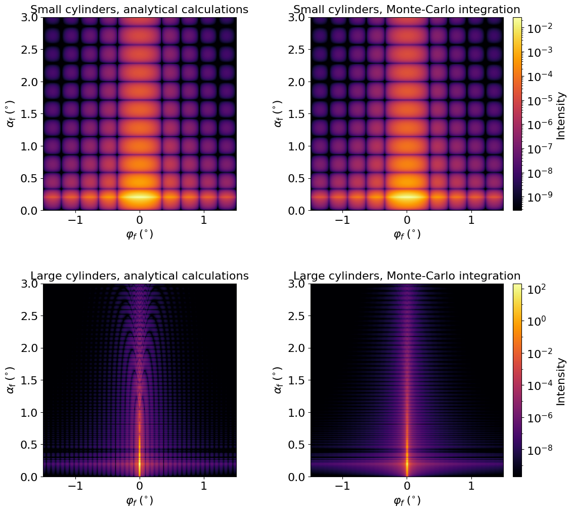
Large cylinders in DWBA.

This example demonstrates that for large particles (~1000nm) the form factor
oscillates rapidly within one detector bin and analytical calculations
(performed for the bin center) give completely wrong intensity pattern.
In this case Monte-Carlo integration over detector bin should be used.
"""
import math

import bornagain as ba
ba.require_versions("bornagain>=25,<26")
from bornagain import angstrom, deg, nm

default_cylinder_radius = 10*nm
default_cylinder_height = 20*nm


def get_sample(cylinder_radius, cylinder_height):
    # Materials
    vacuum = ba.Vacuum()
    substrate_color = (0.28, 0.57, 0.82)
    substrate_mat = ba.RefractiveMaterial("Substrate", substrate_color, 6e-6, 2e-8)
    particle_color = (0.86, 0.24, 0.18)
    particle_mat = ba.RefractiveMaterial("Particle", particle_color, 6e-4, 2e-8)

    # Particle
    ff = ba.Cylinder(cylinder_radius, cylinder_height)
    particle = ba.Particle(particle_mat, ff)

    # Layers
    vacuum_layer = ba.Layer(vacuum)
    # Use dilute 1% areal coverage for both small and large cylinders.
    surface_density = 0.01/(math.pi*cylinder_radius**2)
    vacuum_layer.deposit2D(ba.Dilute2D(surface_density, particle))
    substrate_layer = ba.Layer(substrate_mat)

    # Sample
    sample = ba.Sample()
    sample.addLayer(vacuum_layer)
    sample.addLayer(substrate_layer)
    return sample


def get_simulation(sample, integration_flag):
    """
    A GISAXS simulation with defined beam and detector.
    If integration_flag=True, the simulation will integrate over detector bins.
    """
    beam = ba.Beam(1, 1*angstrom, 0.2*deg)
    n = 201
    det = ba.SphericalDetector(n, -1.5*deg, 1.5*deg, n, 0, 3*deg)
    simulation = ba.ScatteringSimulation(beam, sample, det)
    simulation.options().setMonteCarloIntegration(integration_flag, 50, seed=0)
    if not "__no_terminal__" in globals():
        simulation.setTerminalProgressMonitor()
    return simulation


def simulate():
    ret = []

    # conditions define cylinder scale factor and integration flag
    conditions = [{
        'title': "Small cylinders, analytical calculations",
        'scale': 1,
        'integration': False
    }, {
        'title': "Small cylinders, Monte-Carlo integration",
        'scale': 1,
        'integration': True
    }, {
        'title': "Large cylinders, analytical calculations",
        'scale': 100,
        'integration': False
    }, {
        'title': "Large cylinders, Monte-Carlo integration",
        'scale': 100,
        'integration': True
    }]

    # run simulation 4 times
    for i_plot, condition in enumerate(conditions):
        scale = condition['scale']
        integration_flag = condition['integration']

        sample = get_sample(default_cylinder_radius*scale,
                            default_cylinder_height*scale)
        simulation = get_simulation(sample, integration_flag)
        result = simulation.simulate()
        result.setTitle(condition['title'])
        ret.append(result)

    return ret


if __name__ == '__main__':
    results = simulate()
    sample = get_sample(default_cylinder_radius, default_cylinder_height)
    ba.showSample3D(sample, sample_size=100*nm, seed=199)

    fig, axs = ba.plt.subplots(2, 2, figsize=(12, 10), layout='compressed')
    fig.get_layout_engine().set(wspace=0.12, hspace=0.12)
    small_range = 8
    small_max = max(results[0].intensities().max(),
                    results[1].intensities().max())

    large_range = 12
    large_max = max(results[2].intensities().max(),
                    results[3].intensities().max())

    row_plot_settings = ((small_max, small_range), (large_max, large_range))

    for row, (intensity_max, log_range) in enumerate(row_plot_settings):
        pair = results[2*row:2*row + 2]
        for col, result in enumerate(pair):
            ba.plot_heatmap(
                result,
                ax=axs[row, col],
                title=result.title(),
                zlabel="Intensity",
                intensity_max=intensity_max,
                log_range=log_range,
                unit_aspect=1,
                with_cb=col == 1,
            )

    ba.plt.show()
|