Overview

In fitting, we estimate the optimum parameters in a numerical model, specifically a scattering simulation, by minimizing the difference between simulated and reference data.

BornAgain provides the simulation result. Experimental data import, parameter management, and the residual function are ordinary Python code. This keeps fitting scripts independent of any BornAgain-specific data format and lets users combine BornAgain with standard packages such as numpy, fabio, and lmfit.

In the following we will show how to fit using the BornAgain Python API.

Introductory example

In the following, a very simple example shows how to fit a parametric model to given data.

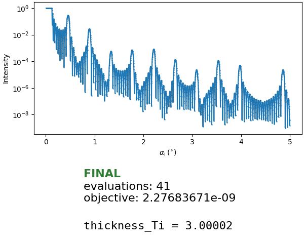
The model is a specular reflectometry scan, with a sample consisting of 20 alternating Ti and Ni layers on a Si substrate. Using this model, synthetic data have been generated with GenX. These data are part of the BornAgain sources, testdata/genx_alternating_layers.dat.gz. The generated example includes a copy beside the script.

From the build directory, run as:

python3 ../auto/Examples/fit/...

The fit model is identical to the model used for generating the data. There is just one fit parameter, namely the thickness of the Ti layers. The resulting fit is indistinguishable from the data:
Script

  1
  2
  3
  4
  5
  6
  7
  8
  9
 10
 11
 12
 13
 14
 15
 16
 17
 18
 19
 20
 21
 22
 23
 24
 25
 26
 27
 28
 29
 30
 31
 32
 33
 34
 35
 36
 37
 38
 39
 40
 41
 42
 43
 44
 45
 46
 47
 48
 49
 50
 51
 52
 53
 54
 55
 56
 57
 58
 59
 60
 61
 62
 63
 64
 65
 66
 67
 68
 69
 70
 71
 72
 73
 74
 75
 76
 77
 78
 79
 80
 81
 82
 83
 84
 85
 86
 87
 88
 89
 90
 91
 92
 93
 94
 95
 96
 97
 98
 99
100
101
102
103
104
105
106
107
108
109
110
111
112
113
#!/usr/bin/env python3
# /// script
# requires-python = ">=3.10"
# dependencies = ["bornagain>=25,<26", "lmfit"]
# ///
"""
Basic example how to fit specular data.
The sample consists of twenty alternating Ti and Ni layers.
Reference data was generated with GenX.
We fit just one parameter, the thickness of the Ti layers,
which has an original value of 30 angstroms.
"""

import bornagain as ba
ba.require_versions("bornagain>=25,<26")
from pathlib import Path
from bornagain import angstrom, nm
import lmfit
import numpy as np


def load_data(filename):
    # Data files are next to this script.
    data_dir = Path(__file__).resolve().parent
    fname = data_dir / filename

    two_alpha, intensity = ba.read_columns(fname, usecols=(0, 1))
    alpha = 0.5*two_alpha*ba.deg
    return alpha, intensity


def datafield_from_arrays(x, y):
    frame = ba.Frame(ba.ListScan("alpha_i (rad)", x))
    return ba.Datafield(frame, y.tolist())


def get_sample(P):
    # Materials
    ti_color = (0.05, 0.62, 0.55)
    ti_mat = ba.SLDMaterial("Ti", ti_color, -1.9493e-06, 0)
    ni_color = (0.93, 0.48, 0.14)
    ni_mat = ba.SLDMaterial("Ni", ni_color, 9.4245e-06, 0)
    si_color = (0.30, 0.62, 0.86)
    si_mat = ba.SLDMaterial("Si", si_color, 2.0704e-06, 0)

    # Layers
    layer_Ti = ba.Layer(ti_mat, P["thickness_Ti"])
    layer_Ni = ba.Layer(ni_mat, 70*angstrom)

    # Periodic stack
    n_repetitions = 10
    stack = ba.LayerStack(n_repetitions)
    stack.addLayer(layer_Ti)
    stack.addLayer(layer_Ni)

    # Sample
    sample = ba.Sample()
    sample.addLayer(ba.Layer(ba.Vacuum()))
    sample.addStack(stack)
    sample.addLayer(ba.Layer(si_mat))

    return sample


def get_simulation(alpha_axis, P):
    scan = ba.AlphaScan(alpha_axis)
    scan.setWavelength(1.54*angstrom)
    sample = get_sample(P)

    return ba.SpecularSimulation(scan, sample)


if __name__ == '__main__':
    alpha, exp_values = load_data("genx_alternating_layers.dat.gz")
    exp_data = datafield_from_arrays(alpha, exp_values)

    # Fit progress display
    fit_plotter = ba.FitPlotter(
        ba.plot_specular,
        context_data=exp_data,
        ylabel="Intensity",
    )

    monitor = ba.FitMonitor(
        fit_plotter,
        ncols=1,
        show_best=True,
        max_fps=1,
        printer=ba.Printer(every_nth=10),
        live=True)

    def residuals(P):
        """
        Simulates, reports, and returns the residual vector.
        """
        sim_result = get_simulation(alpha, P.valuesdict()).simulate()
        residuals = exp_values - sim_result.intensities()
        monitor.update(sim_result, P, residuals)
        return residuals

    P = lmfit.Parameters()
    P.add("thickness_Ti", value=5*nm, min=1*nm, max=6*nm)

    result = lmfit.minimize(residuals, P, method="leastsq")

    finalP = result.params.valuesdict()
    # Recompute and report the simulation at the fitted parameters.
    residuals(result.params)
    # Render the just-reported evaluation as the final fit state.
    monitor.render_final(result.params)
    print(lmfit.fit_report(result))
    ba.showSample3D(get_sample(finalP), sample_size=120*nm, seed=0)
    ba.plt.show()
auto/Examples/fit/specular/Specular1Par.py

Explanations

The arrays alpha and exp_values contain the data to be fitted. They are read with ba.read_columns and converted explicitly to the units required by the simulation; see Data import.

The lmfit.Parameters object P contains the fit parameters. The function residuals(P) is passed to the minimizer. It converts the lmfit parameters to a plain dictionary, runs the BornAgain simulation, extracts simulated intensities as a NumPy array, reports the completed evaluation, and returns the residual vector.

FitPlotter describes one subplot by combining a plotting function, optional fixed plot data, and plotting arguments. FitMonitor arranges one or more such plots and adds the fit status. The residual function reports each complete evaluation directly:

# Fit progress display
fit_plotter = ba.FitPlotter(
    ba.plot_specular,
    context_data=exp_data,
    ylabel="Intensity",
)

monitor = ba.FitMonitor(
    fit_plotter,
    ncols=1,
    show_best=True,
    max_fps=1,
    printer=ba.Printer(every_nth=10))

def residuals(P):
    simulation = get_simulation(alpha, P.valuesdict()).simulate()
    residuals = exp_values - simulation.intensities()
    monitor.update(simulation, P, residuals)
    return residuals

result = lmfit.minimize(residuals, P, method="leastsq")
# Recompute and report the simulation at the fitted parameters.
residuals(result.params)
# Render the just-reported evaluation as the final fit state.
monitor.render_final(result.params)
ba.plt.show()

Here exp_data remains fixed as the plotter’s context_data, while monitor.update(simulation, P, residuals) supplies one complete evaluation. The standard plot_specular helper draws the measured and simulated curves on the subplot managed by FitMonitor. max_fps limits graphical redraws, independently of the evaluation interval selected by Printer.every_nth for terminal output. The explicit final residual call evaluates the fitted parameters through this same update path before render_final renders them.

A custom plotting function receives the current result first: plotter_fn(result, ax=subplot, **plot_args). If context_data is configured, the monitor also passes it as a keyword argument. This is fixed data for that plot, not sample or detector configuration and not fit state. The result may also be a tuple of simulations. This keeps standard BornAgain plots and user-defined derived plots equally usable without requiring source callbacks. For its complete optimizer-independent interface, constructor parameters, layout, and display helpers, see Fit reference > Fit monitoring.

For masked detector pixels, BornAgain simulations return NaN. Residual functions that use detector masks should exclude those entries explicitly. The helper ba.valid_pixel_residual(exp, sim) does this and also excludes non-finite or negative experimental values, the dead-pixel markers of real detectors.

For a rectangular analysis window described by a boolean detector mask, ba.crop_by_mask(data, mask) returns the part of the data inside the smallest rectangle containing all unmasked (False) pixels.