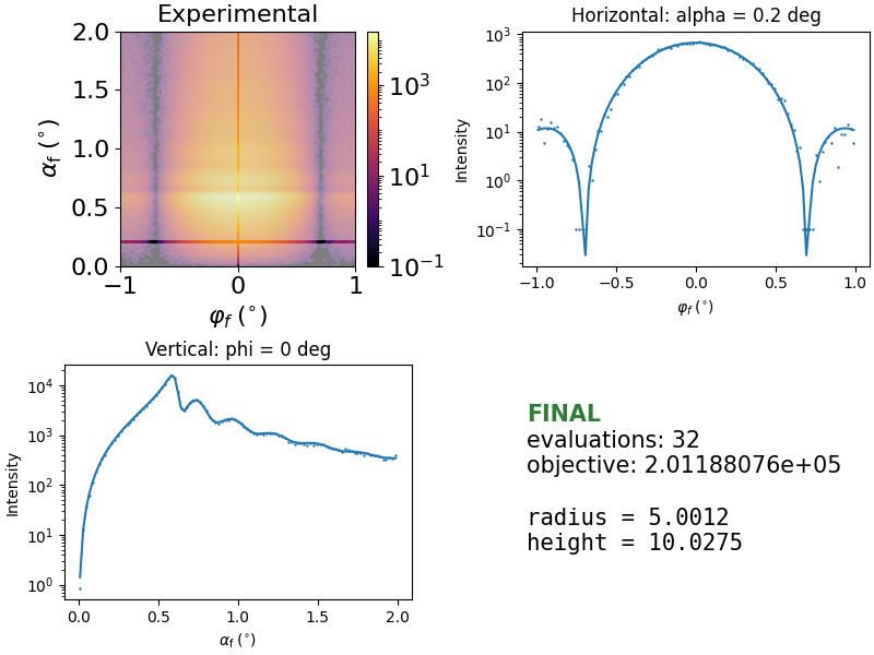
1
  2
  3
  4
  5
  6
  7
  8
  9
 10
 11
 12
 13
 14
 15
 16
 17
 18
 19
 20
 21
 22
 23
 24
 25
 26
 27
 28
 29
 30
 31
 32
 33
 34
 35
 36
 37
 38
 39
 40
 41
 42
 43
 44
 45
 46
 47
 48
 49
 50
 51
 52
 53
 54
 55
 56
 57
 58
 59
 60
 61
 62
 63
 64
 65
 66
 67
 68
 69
 70
 71
 72
 73
 74
 75
 76
 77
 78
 79
 80
 81
 82
 83
 84
 85
 86
 87
 88
 89
 90
 91
 92
 93
 94
 95
 96
 97
 98
 99
100
101
102
103
104
105
106
107
108
109
110
111
112
113
114
115
116
117
118
119
120
121
122
123
124
125
126
127
128
129
130
131
132
133
134
135
136
137
138
139
140
141
142
143
144
145
146
147
148
149
150
151
152
153
154
155
156
157
158
159
160
161
162
163
164
165
166
167
168
169
170
171
172
173
174
175
176
177
178
179
180
181
182
183
184
185
186
187
188
189
190
191
192
193
194
195
196
197
198
199
200
201
202
|
#!/usr/bin/env python3
# /// script
# requires-python = ">=3.10"
# dependencies = ["bornagain>=25,<26", "lmfit"]
# ///
"""
Fitting example: fit along slices
"""

import bornagain as ba
ba.require_versions("bornagain>=25,<26")
from bornagain import deg, nm, nm2
import lmfit
import numpy as np


def get_sample(P):
    """
    Uncorrelated cylinders on a substrate, parameterized for fitting.
    """
    substrate_color = (0.28, 0.57, 0.82)
    particle_color = (0.86, 0.24, 0.18)

    substrate_mat = ba.RefractiveMaterial("Substrate", substrate_color, 6e-6, 2e-8)
    particle_mat = ba.RefractiveMaterial("Particle", particle_color, 6e-4, 2e-8)
    particle = ba.Particle(particle_mat, ba.Cylinder(P["radius"], P["height"]))

    particle_layer = ba.Layer(ba.Vacuum())
    # Modest coverage keeps material averaging physical over the fit bounds.
    particle_layer.deposit2D(ba.Dilute2D(1e-3/nm2, particle))

    sample = ba.Sample()
    sample.addLayer(particle_layer)
    sample.addLayer(ba.Layer(substrate_mat))
    return sample


def get_simulation(P):
    """
    GISAS simulation for the parameterized cylinder sample.
    """
    n = 101
    beam = ba.Beam(1e8, 0.1*nm, 0.2*deg)
    detector = ba.SphericalDetector(n, -1*deg, 1*deg, n, 0, 2*deg)
    simulation = ba.ScatteringSimulation(beam, get_sample(P), detector)
    return simulation


phi_slice_value = 0.0  # position of vertical slice in deg
alpha_slice_value = 0.2  # position of horizontal slice in deg


def closest_axis_index(axis, value):
    centers = np.asarray(axis.binCenters())
    return int(np.argmin(np.abs(centers - value)))


def data_slice(data, axis_index, fixed_index):
    """
    Returns one horizontal or vertical detector slice as a 1D Datafield.
    """
    data = data.plottableField()
    values = (data.intensities()[fixed_index, :]
              if axis_index == 0 else
              data.intensities()[:, fixed_index])
    axis = data.axis(axis_index)
    scale = ba.ListScan(axis.axisLabel(), list(axis.binCenters()))
    return ba.Datafield(ba.Frame(scale), values.tolist())


def slice_curves(experimental, simulated, axis_index, fixed_index):
    """
    Returns measured and simulated Datafields for one detector slice.
    """
    return [("Slice",
             data_slice(experimental, axis_index, fixed_index),
             data_slice(simulated, axis_index, fixed_index))]


def plot_slice(simulation, ax=None, *, context_data, axis_index, fixed_index,
               title):
    """
    Plots one measured and simulated detector slice.
    """
    curves = slice_curves(
        context_data, simulation, axis_index, fixed_index)
    ba.plot_specular_curves(curves, ax=ax, ylabel="Intensity")
    ax.set_title(title)


def get_masked_simulation(P):
    """
    GISAS simulation with only one horizontal and one vertical slice active.
    """
    n = 101
    beam = ba.Beam(1e8, 0.1*nm, 0.2*deg)
    sample = get_sample(P)
    detector = ba.SphericalDetector(n, -1*deg, 1*deg, n, 0, 2*deg)
    n_phi = detector.axis(0).size()
    n_alpha = detector.axis(1).size()

    mask = np.ones((n_alpha, n_phi), dtype=bool)
    i_phi = closest_axis_index(detector.axis(0), phi_slice_value*deg)
    i_alpha = closest_axis_index(detector.axis(1), alpha_slice_value*deg)
    mask[:, i_phi] = False
    mask[i_alpha, :] = False
    detector.setMask(mask)

    simulation = ba.ScatteringSimulation(beam, sample, detector)
    return simulation


def fake_data():
    """
    Generating "real" data by adding noise to the simulated data.
    """
    # initial values which we will have to find later during the fit
    P = {'radius': 5*nm, 'height': 10*nm}

    simulation = get_simulation(P)
    simulation.setBackground(ba.PoissonBackground(seed=0))
    result = simulation.simulate()

    return result.noisy(0.1, 0.1)


def get_plotters(exp_data):
    """
    Creates the detector-map and slice plotters.
    """
    i_phi = closest_axis_index(exp_data.axis(0), phi_slice_value*deg)
    i_alpha = closest_axis_index(exp_data.axis(1), alpha_slice_value*deg)
    norm = ba.intensity_norm(exp_data)

    experiment_plotter = ba.FitPlotter(
        ba.plot_masked_experimental,
        context_data=exp_data,
        norm=norm,
        with_cb=True,
        title="Experimental",
    )

    horizontal_slice_plotter = ba.FitPlotter(
        plot_slice,
        context_data=exp_data,
        axis_index=0,
        fixed_index=i_alpha,
        title=f"Horizontal: alpha = {alpha_slice_value:g} deg",
    )

    vertical_slice_plotter = ba.FitPlotter(
        plot_slice,
        context_data=exp_data,
        axis_index=1,
        fixed_index=i_phi,
        title=f"Vertical: phi = {phi_slice_value:g} deg",
    )

    return [
        experiment_plotter,
        horizontal_slice_plotter,
        vertical_slice_plotter,
    ]


if __name__ == '__main__':
    exp_data = fake_data()
    exp_values = exp_data.intensities()

    # Fit progress display
    monitor = ba.FitMonitor(
        get_plotters(exp_data),
        ncols=2,
        show_best=True,
        max_fps=1,
        printer=ba.Printer(every_nth=10),
        live=True)

    def residuals(P):
        """
        Simulates and reports residuals; masked pixels contribute zero.
        """
        sim_result = get_masked_simulation(P.valuesdict()).simulate()
        residuals = ba.valid_pixel_residual(exp_values,
                                                sim_result.intensities())
        monitor.update(sim_result, P, residuals)
        return residuals

    P = lmfit.Parameters()
    P.add("radius", value=6*nm, min=4*nm, max=8*nm)
    P.add("height", value=9*nm, min=8*nm, max=12*nm)

    result = lmfit.minimize(residuals, P, method="leastsq")

    finalP = result.params.valuesdict()
    # Recompute and report the simulation at the fitted parameters.
    residuals(result.params)
    # Render the just-reported evaluation as the final fit state.
    monitor.render_final(result.params)
    print(lmfit.fit_report(result))
    ba.showSample3D(get_sample(finalP), sample_size=120*nm, seed=0)
    ba.plt.show()
|