 BornAgain
≻ git-develop
≻ Documentation ≻ Reference ≻ Simulation model ≻ Common settings ≻ Background
BornAgain
≻ git-develop
≻ Documentation ≻ Reference ≻ Simulation model ≻ Common settings ≻ Background
BornAgain
≻ git-develop
≻ Documentation ≻ Reference ≻ Simulation model ≻ Common settings ≻ Background
BornAgain
≻ git-develop
≻ Documentation ≻ Reference ≻ Simulation model ≻ Common settings ≻ Background
To add a Poisson background to a Simulation instance, use
bg = ba.PoissonBackground(seed=0)
simulation.setBackground(bg)
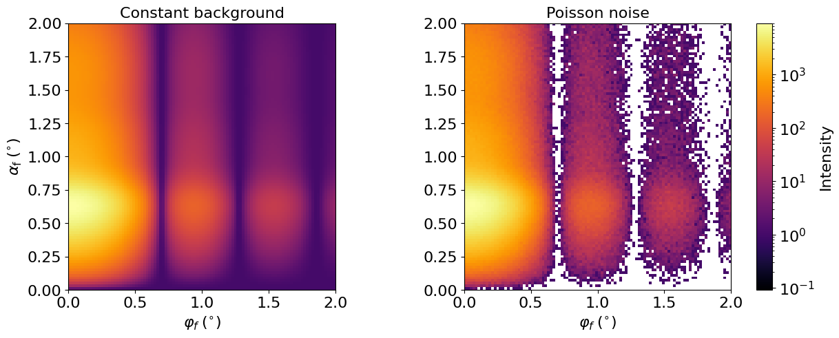
In this case, the output intensity is randomly distributed around the exact value with discrete Poisson statistics. The same seed reproduces the same noise realization.
The lower the intensity of the probing beam, the lower the signal-to-noise ratio.
To add a constant background to a Simulation instance, use
bg = ba.ConstantBackground(1e3)
simulation.setBackground(bg)
A Python object with a background method can transform the complete simulated
field. The method receives the original Datafield and returns a new
Datafield with the same frame. For example, a specular scan assembled from
two exposure regions can use
class StitchedBackground:
    def __init__(self, boundary, left, right):
        self.boundary = boundary
        self.left = left
        self.right = right

    def background(self, field):
        x = np.asarray(field.xCenters())
        added = np.where(x < self.boundary, self.left, self.right)
        values = field.intensities() + added
        return ba.Datafield(field.title(), field.frame(), values.tolist())


bg = StitchedBackground(boundary=0.5*deg, left=20., right=100.)
simulation.setBackground(bg)
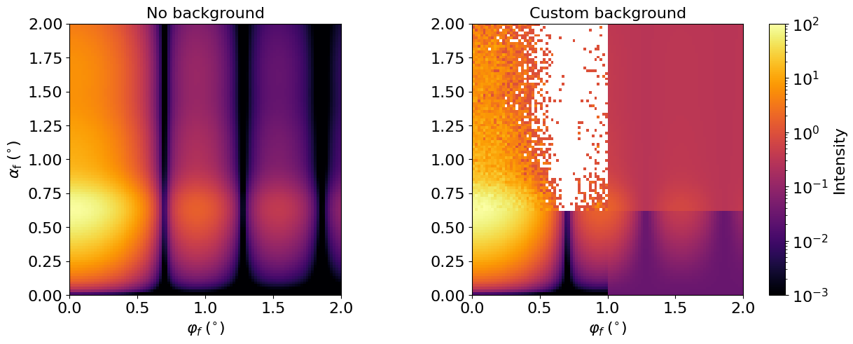
The input field provides the original intensities and all output-bin coordinates. A two-dimensional coordinate-dependent background can use
class CustomBackground:
    def background(self, field):
        x = np.asarray(field.xCenters())
        y = np.asarray(field.yCenters())
        values = field.intensities()
        values = values + 5. + 2.*x[np.newaxis, :] + 3.*y[:, np.newaxis]
        return ba.Datafield(field.title(), field.frame(),
                            values.ravel().tolist())
The callback is invoked after the scattering calculation. Its result must preserve the input frame and masked bins and contain finite, nonnegative intensities in all computed bins. This makes it suitable for interpolation of a measured background map without restricting the number of simulation threads.
Specular simulation also transforms a zero field to obtain the background baseline used by its normalization. For an additive background (B(x)), a simulated reflected intensity (I(x)), and probe beam intensity (I_0), the result is ((I(x) + B(x)) / (I_0 + B(x))).
Background is not supported.
The specular Background example compares constant background with Poisson noise in a reflectometry scan.
Scattering intensity
Coordinate-dependent background
The GISAS script shows the same built-in constant and Poisson backgrounds.
The second script compares a simulation without background to one using a Python-defined background for four detector regions.