In this example we simulate the scattering from a one-dimensional repetition
of rectangular patches. This is done by using Crystal1D together with very
long boxes.
length, width, height in the Box(length, width, height) constructor
correspond to the $x$, $y$, $z$ axes, in that order.Crystal1D lattice direction
and the particle.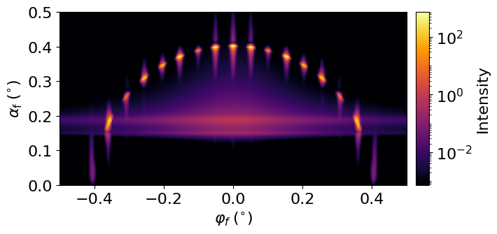
Scattering intensity
|
|
A one-dimensional lattice can be viewed as a chain of particles placed at regular intervals on a single axis. One use case is a grating, where very long boxes are placed at nodes of a 1D lattice.
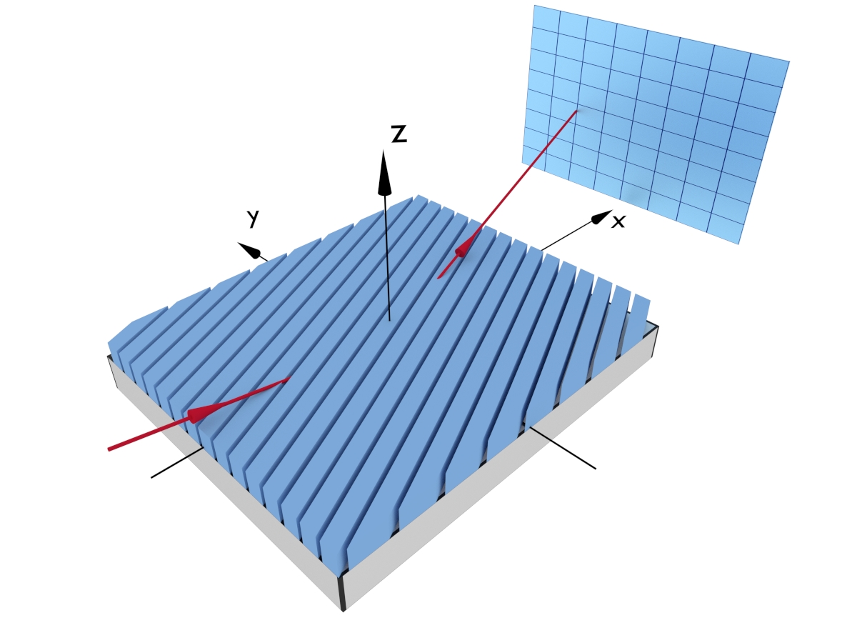
See the BornAgain user manual (Chapter 3.4.1, One Dimensional Lattice) for details about the theory.
The structure is created with
structure = ba.Crystal1D(particle, length, xi, linear_density)
Arguments:
particle        # particle or Mixture placed at lattice sites
length          # lattice constant, in nanometers
xi              # rotation of the lattice with respect to x-axis, in radians
linear_density  # number of lattice lines per nanometer in the transverse axis
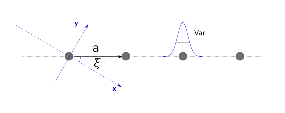
When the beam azimuthal angle $\varphi_f$ is zero, the beam direction coincides with x-axis. In this case, $\xi$ can be considered as the lattice rotation with respect to the beam.
The position variance parameter allows uncertainty for each particle position around the lattice point by applying a corresponding Debye-Waller factor.
It can be set using the setLateralPositionVariance(value) method, where
value is given in nm$^2$.
structure = ba.Crystal1D(particle, 100*nm, 0*deg, 1/box_length)
structure.setLateralPositionVariance(0.1)
By default the variance is set to zero.
To account for finite size effects of the lattice, assign a decay function to the structure. This function encodes the loss of coherent scattering from lattice points with increasing distance between them. The origin of this loss of coherence could be attributed to the coherence length of the beam or to the domain structure of the lattice.
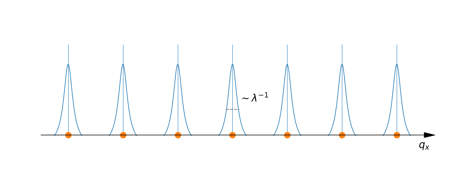
In the picture below a one-dimensional lattice is represented in real space as a probability density function for finding a particle at a given coordinate on the x-axis. In the presence of a decay function, this density can be given as $\sum F_{decay}(x)\cdot\delta(x-na)$.
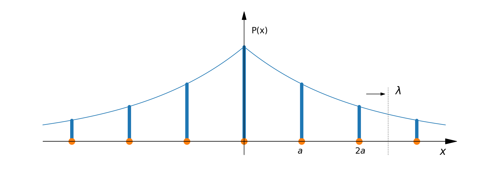
The Fourier transform of this distribution $P(x)$ provides the scattering amplitude in reciprocal space. An exponential decay law in real space with the decay length $\lambda$ will give a Cauchy distribution with characteristic width $1/\lambda$ in reciprocal space, as shown below.
The decay function is assigned with setDecayFunction(decay):
structure = ba.Crystal1D(particle, 10*nm, 0*deg, 1/box_length)
structure.setDecayFunction(ba.Profile1DCauchy(1000*nm))
BornAgain supports four types of one-dimensional decay functions.
Profile1DCauchy(decay_length): one-dimensional Cauchy decay function in
reciprocal space, corresponding to $exp(-|x|/\lambda)$ in real space.Profile1DGauss(decay_length): one-dimensional Gauss decay function in
reciprocal space, corresponding to $exp(-x^2/(2*\lambda^2))$ in real space.Profile1DTriangle(decay_length): one-dimensional triangle decay function
in reciprocal space, corresponding to $1-|x|/\lambda$ if $|x|<\lambda$ in
real space.Profile1DVoigt(decay_length, eta): one-dimensional pseudo-Voigt decay
function in reciprocal space, corresponding to
$eta*Gauss + (1-eta)*Cauchy$.The parameter $\lambda$ is given in nanometers and sets the characteristic
length scale at which loss of coherence takes place. In the case of the
pseudo-Voigt distribution, an additional dimensionless parameter eta
balances between the Gaussian and Cauchy profiles.
The linear_density constructor argument gives the number of lattice lines per
nanometer in the direction transverse to the 1D lattice. For a grating made of
long boxes, use the inverse box length.
The rotation of the lattice does not change the orientation of the particles with respect to the beam direction. To rotate a grating as a physical object, rotate both the particle and the lattice direction.
For example:
box = ba.Particle(material, ba.Box(10*nm, 1000*nm, 10*nm))
box.rotate(ba.RotationZ(30*deg))

structure = ba.Crystal1D(box, 40*nm, 30*deg, 1/(1000*nm))
layer.deposit2D(structure)