Bayesian sampling

Bayesian sampling of reflectometry models is a common tool in the analysis of specular reflectometry data. The Python programming language has a powerful infrastructure for this modelling, including packages such as PyMC3 and PyStan. Here, we show how emcee enables Bayesian sampling in BornAgain. The initial maximum-likelihood estimate uses the differential evolution algorithm exposed by lmfit.

Example script

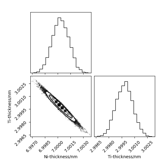
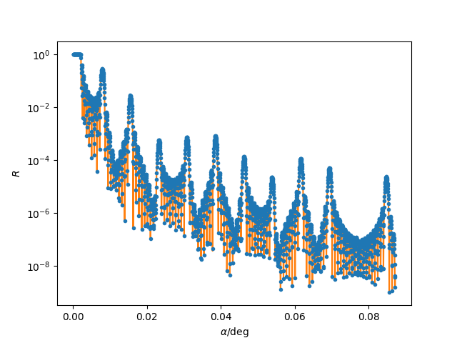
To generate these images of the probability distributions of the parameters and the maximum likelihood reflectometry profile
run this script

  1
  2
  3
  4
  5
  6
  7
  8
  9
 10
 11
 12
 13
 14
 15
 16
 17
 18
 19
 20
 21
 22
 23
 24
 25
 26
 27
 28
 29
 30
 31
 32
 33
 34
 35
 36
 37
 38
 39
 40
 41
 42
 43
 44
 45
 46
 47
 48
 49
 50
 51
 52
 53
 54
 55
 56
 57
 58
 59
 60
 61
 62
 63
 64
 65
 66
 67
 68
 69
 70
 71
 72
 73
 74
 75
 76
 77
 78
 79
 80
 81
 82
 83
 84
 85
 86
 87
 88
 89
 90
 91
 92
 93
 94
 95
 96
 97
 98
 99
100
101
102
103
104
105
106
107
108
109
110
111
112
113
114
115
116
117
118
119
120
121
122
123
124
125
126
127
128
129
130
131
132
133
134
135
136
137
138
139
140
141
142
143
144
145
146
147
148
149
150
151
152
153
154
155
156
157
158
159
#!/usr/bin/env python3
# /// script
# requires-python = ">=3.10"
# dependencies = ["bornagain>=25,<26", "corner", "emcee", "lmfit"]
# ///
"""
An example of using the Bayesian sampling library emcee with BornAgain.

Author: Andrew McCluskey (andrew.mccluskey@ess.eu)
"""

from itertools import count
import os

import bornagain as ba
ba.require_versions("bornagain>=25,<26")
import corner
import emcee
import lmfit
import matplotlib.pyplot as plt
import numpy as np
from bornagain import ba_io, nm


np.random.seed(1)

datadir = ba_io.data_dir()


def get_sample(ni_thickness, ti_thickness):
    # pure real scattering-length densities (in angstrom^-2)
    si_sld_real = 2.0704e-06  # Si (substrate)
    ni_sld_real = 9.4245e-06  # Ni
    ti_sld_real = -1.9493e-06  # Ti

    # materials
    vacuum = ba.Vacuum()
    ni_color = (0.93, 0.48, 0.14)
    ni_mat = ba.SLDMaterial("Ni", ni_color, ni_sld_real, 0)
    ti_color = (0.05, 0.62, 0.55)
    ti_mat = ba.SLDMaterial("Ti", ti_color, ti_sld_real, 0)
    substrate_color = (0.28, 0.57, 0.82)
    substrate_mat = ba.SLDMaterial("SiSubstrate", substrate_color, si_sld_real, 0)

    # layers
    vacuum_layer = ba.Layer(vacuum)
    ni_layer = ba.Layer(ni_mat, ni_thickness)
    ti_layer = ba.Layer(ti_mat, ti_thickness)
    substrate_layer = ba.Layer(substrate_mat)

    # periodic stack
    n_repetitions = 10
    stack = ba.LayerStack(n_repetitions)
    stack.addLayer(ti_layer)
    stack.addLayer(ni_layer)

    # sample
    sample = ba.Sample()
    sample.addLayer(vacuum_layer)
    sample.addStack(stack)
    sample.addLayer(substrate_layer)

    return sample


def get_simulation(sample, points):
    scan = ba.AlphaScan(ba.ListScan("alpha_i (rad)", points))
    scan.setWavelength(0.154 * nm);
    return ba.SpecularSimulation(scan, sample)


def run_simulation(points, ni_thickness, ti_thickness):
    sample = get_sample(ni_thickness, ti_thickness)
    simulation = get_simulation(sample, points)

    result = simulation.simulate()
    return result.intensities()


if __name__ == '__main__':
    filepath = os.path.join(datadir, "specular/genx_alternating_layers.dat.gz")
    two_alpha, y = ba_io.read_columns(filepath, usecols=(0, 1))
    q = 0.5*two_alpha*ba.deg
    dy = y * 0.1 # arbitrary uncertainties

    def log_likelihood(P):
        """
        Calculates the log-likelihood for the normal uncertainties
        :tuple sim_var: the variable parameters
        :array x: the abscissa data (q-values)
        :array y: the ordinate data (R-values)
        :array yerr: the ordinate uncertainty (dR-values)
        :return: log-likelihood
        """
        y_sim = run_simulation(q, *P)
        sigma2 = dy**2 + y_sim**2
        return -0.5*np.sum((y - y_sim)**2/sigma2 + np.log(sigma2))

    def de_objective(P):
        values = [P["ni_thickness"].value, P["ti_thickness"].value]
        return -log_likelihood(values)

    parameters = lmfit.Parameters()
    parameters.add("ni_thickness", value=7*nm, min=5*nm, max=9*nm)
    parameters.add("ti_thickness", value=5.5*nm, min=1*nm, max=10*nm)
    n_generations = 1000
    generations = count(1)

    def stop_callback(*_args, **_kwargs):
        return next(generations) >= n_generations

    # Each generation uses 15*2 likelihood evaluations; the emergency cap
    # must also cover the initial population and polishing.
    solution = lmfit.minimize(
        de_objective,
        parameters,
        method="differential_evolution",
        callback=stop_callback,  # stops the search after n_generations
        popsize=15,
        max_nfev=100000,  # emergency evaluation cap
        polish=True,
        seed=42)

    best_ni_thickness = solution.params["ni_thickness"].value
    best_ti_thickness = solution.params["ti_thickness"].value
    best_fit = np.array([best_ni_thickness, best_ti_thickness])
    print('MLE Ni Thickness', best_ni_thickness, 'nm')
    print('MLE Ti Thickness', best_ti_thickness, 'nm')

    # Perform the likelihood sampling
    n_walkers = 32
    n_parameters = best_fit.size
    walker_spread = 1e-4
    walker_positions = np.random.normal(
        best_fit, walker_spread, (n_walkers, n_parameters))
    sampler = emcee.EnsembleSampler(n_walkers, n_parameters, log_likelihood)
    sampler.run_mcmc(walker_positions,
                     1000,
                     progress=True)

    # Plot and show corner plot of samples
    flat_samples = sampler.get_chain(flat=True)
    corner.corner(flat_samples,
                  labels=['Ni-thickness/nm', 'Ti-thickness/nm'])
    plt.show()

    sample = get_sample(*flat_samples.mean(axis=0))
    ba.showSample3D(sample, sample_size=120*nm, seed=0)

    # Plot and show MLE and data of reflectivity
    plt.errorbar(q, y, dy, marker='.', ls='')
    plt.plot(
        q,
        run_simulation(q, *flat_samples.mean(axis=0)),
        '-')
    plt.xlabel('$\\alpha$/rad')
    plt.ylabel('$R$')
    plt.yscale('log')
    plt.show()
auto/Examples/bayesian/likelihood_sampling.py

Explanation

The system under investigation in the above example is a Ni-Ti multilayer material at the interface between an Si substrate and a vacuum. There are two parameters of interest, the thicknesses of the Ni and Ti layers. We know the scattering length densities for each, and that in total there are 10 repetitions of the Ni-Ti sandwich. This sample is created in the get_sample function.

Having built the sample, it is necessary to obtain the real experimental data. This example requires the data file genx_alternating_layers.dat.gz

from the BornAgain repository.

The environment variable BA_DATA_DIR must point to the testdata/ directory. From the build directory, run:

BA_DATA_DIR=../testdata python3 ../auto/Examples/bayesian/likelihood_sampling.py

The get_real_data function defines an uncertainty in the reflectivity of 10 %.

The simulation is then defined in the get_simulation function, which is passed a series of angles, however, this may be modified to perform a Q-scan as necessary. The final function that is necessary is the simulation of specular reflectometry is the run_simulation function. This will take the angle-value to be simulated and thickness for the Ni and Ti layers and then return the result of the simulation as a numpy.array.

We use the emcee package to sample the likelihood of the data, following its data fitting example. Therefore, it is necessary to define a likelihood (the log_likelihood function) objective. Then, within the main body of the script, we first find the maximum likelihood solution using differential evolution through lmfit.minimize. This should print thicknesses around 7 nm and 3 nm for Ni and Ti, respectively.

We can use the emcee.EnsembleSampler to probe the parameter uncertainties and their correlation. This will perform the sampling for some time (on my machine it took about 2.5 minutes to sample 1000 steps with 32 walkers). Having collected the samples, we can then unpack them and using the corner package visualise them. This will give the first image shown above.

Finally, we can plot the maximum likelihood estimate for the model along with the experimental data. This is the second image above.

Note that the flat_samples object describes the distributions shown in the corner plot. Therefore we can find values of interest, such as the standard deviation or confident intervals.