This is an example of a real data fit. We use our own measurements performed at the laboratory diffractometer GALAXI in Forschungszentrum Jülich.
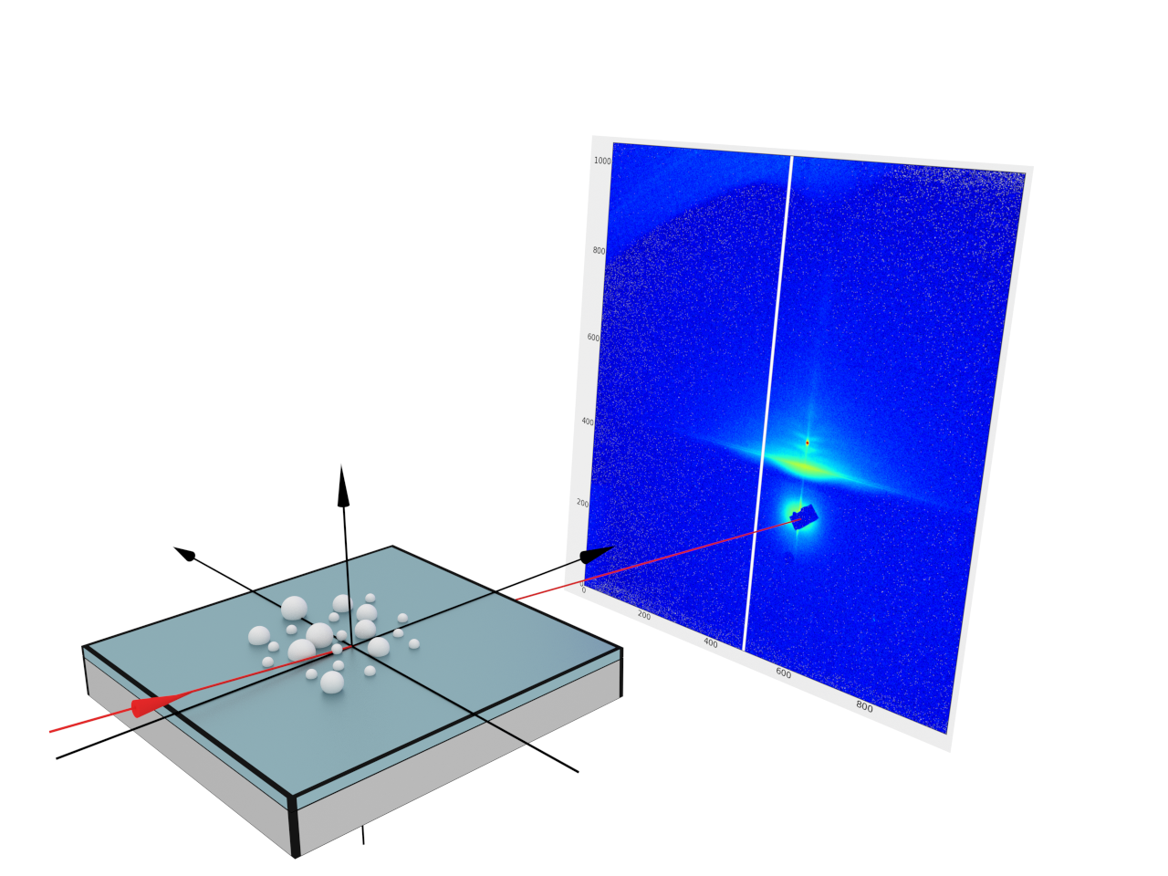
Real-space model

Historical fit (BornAgain 1.19)
Mixture of spheres with different radii.CommonDepthCrosscorrelation vertically correlates the upper interfaces
with the interface below, producing the roughness-interference contribution
alongside the particle scattering.NaN in the simulation result and are not computed.FitPlotter objects show the experimental data, model, and relative
difference. FitMonitor displays the best evaluation during fitting and
renders the explicit final model below.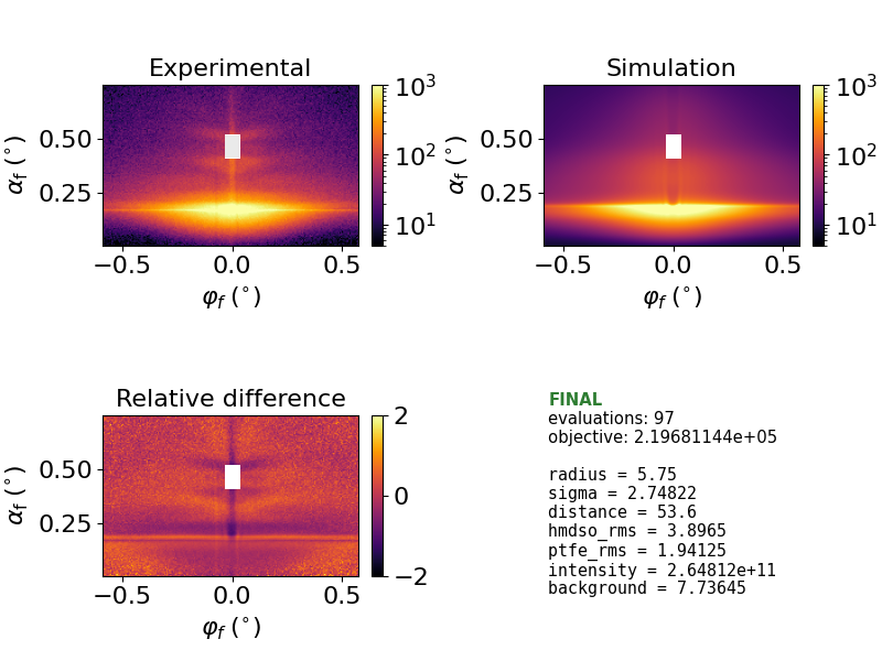
Final BornAgain 25 fit
To successfully simulate and fit results of some real experiment it is important to have
As an example we will use our own measurements performed at the laboratory diffractometer GALAXI in Forschungszentrum Jülich.
Our sample represents a 4-layer system (substrate, teflon, hmdso and air) with Ag nanoparticles embedded in the hmdso layer, on top of the teflon layer. The PILATUS 1M detector was placed at a distance of 1730 mm from the sample.
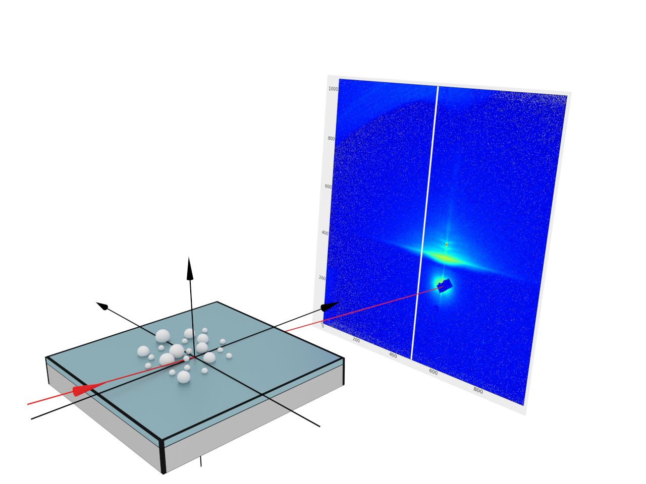
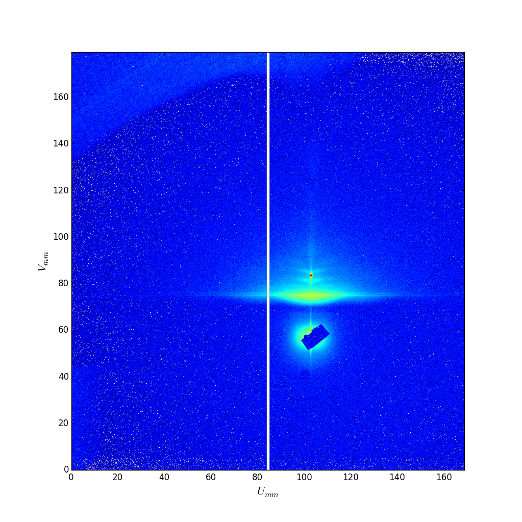
The results of the measurement are represented by the intensity image taken in certain conditions (beam wavelength, grazing angle, detector angular range) and stored in a 32-bit tiff file. To be able to fit these data we have to
From the experimental setup we know the pixel size, the sample-detector distance, and the point where the direct beam hits the detector. A helper function converts the selected pixel edges on the flat detector to scattering angles in radians:
def detector_angle_range(pixel_centers, pixel_size, beam_position,
                         detector_distance, beam_center_angle):
    def detector_angle(position):
        return (np.arctan2(position - beam_position, detector_distance)
                + beam_center_angle)

    lower_edge = pixel_centers[0] - pixel_size/2
    upper_edge = pixel_centers[-1] + pixel_size/2
    return detector_angle(lower_edge), detector_angle(upper_edge)
At the direct-beam position, the azimuth is zero and the exit angle is
-alpha_i. The masks and detector are then constructed explicitly from
the calibrated coordinates:
full_nx = 981
full_ny = 1043
pixel_size = 0.172  # in mm
detector_distance = 1730  # in mm
beam_x_pixel_pos, beam_y_pixel_pos = 597.1, 323.4  # from lower left
alpha_i = 0.463*deg

x_pixels = (np.arange(full_nx) + 0.5)*pixel_size
y_pixels = (np.arange(full_ny) + 0.5)*pixel_size
x_grid, y_grid = np.meshgrid(x_pixels, y_pixels)
inside_window = ((x_grid > 85) & (x_grid < 120)
                 & (y_grid > 70) & (y_grid < 92))
window_mask = np.logical_not(inside_window)
fit_x = ba.crop_by_mask(x_grid, window_mask)
fit_y = ba.crop_by_mask(y_grid, window_mask)

beam_x_pos = beam_x_pixel_pos*pixel_size
beam_y_pos = beam_y_pixel_pos*pixel_size
phi_min, phi_max = detector_angle_range(
    fit_x[0, :], pixel_size, beam_x_pos, detector_distance, 0)
alpha_min, alpha_max = detector_angle_range(
    fit_y[:, 0], pixel_size, beam_y_pos, detector_distance, -alpha_i)

specular_beam_mask = ((fit_x > 101.9) & (fit_x < 103.7)
                      & (fit_y > 82.1) & (fit_y < 85.2))

cropped_ny, cropped_nx = fit_x.shape
detector = ba.SphericalDetector(
    cropped_nx, phi_min, phi_max,
    cropped_ny, alpha_min, alpha_max)
detector.setMask(specular_beam_mask)
The fit window and specular-beam exclusion remain in millimeters, matching
their experimental specification. ba.crop_by_mask follows the
detector mask convention: True marks excluded pixels. It returns the part
of the data inside the smallest rectangle containing every unmasked pixel.
The experimental array is cropped to the fit window before fitting. A spherical detector with the same number of pixels and angular boundaries then approximates this part of the flat detector to a fraction of a pixel.
After cropping, a boolean bitmap mask excludes the specular beam.
The mask shape is (n_alpha, n_phi) and True marks excluded pixels.
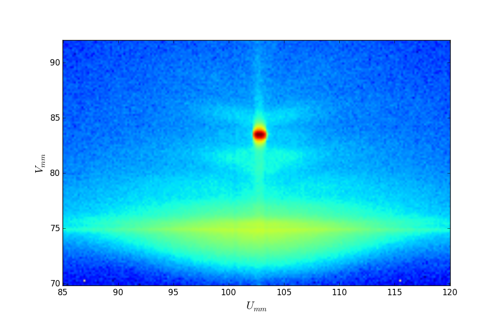
The final simulation setup looks as follows:
beam = ba.Beam(P["intensity"], 1.34*angstrom, alpha_i)
sample = get_sample(P)
simulation = ba.ScatteringSimulation(beam, sample, detector)
During the fit, masked detector pixels are stored as NaN in the
simulation result. The residual function therefore only reads the
unmasked pixels, and additionally skips the negative dead-pixel
markers of the PILATUS image.
The Fabio library provides a convenient way to import experimental data in the form of a numpy array.
import fabio

img = fabio.open("galaxi_data.tif.gz")
data = np.flipud(img.data.astype("float64"))
data = ba.crop_by_mask(data, window_mask)
The full image has shape (1043, 981). After np.flipud, the fit
window is selected by the boolean mask and has the same shape as the
cropped detector, (128, 204). Note that fabio returns the image with
row 0 at the top detector row, whereas BornAgain expects row 0 at the
smallest scattering angle.
|
|
Data to be fitted: galaxi_data.tif.gz
