1
2
3
4
5
6
7
8
9
10
11
12
13
14
15
16
17
18
19
20
21
22
23
24
25
26
27
28
29
30
31
32
33
34
35
36
37
38
39
40
41
42
43
44
45
46
47
48
49
50
51
52
53
54
55
56
57
58
59
60
61
62
63
64
65
66
67
68
69
70
71
72
73
74
75
76
77
78
79
80
81
82
83
84
85
86
87
88
89
90
91
92
93
94
95
96
97
98
99
100
101
102
103
104
105
106
107
108
109
110
111
112
113
114
115
116
117
118
119
120
121
122
123
124
125
126
127
128
129
130
131
132
133
134
135
136
137
138
139
140
141
142
143
144
145
146
147
148
149
150
151
152
153
154
155
156
157
158
159
160
161
162
163
164
165
166
167
168
169
170
171
172
173
174
175
176
177
178
179
180
181
182
183
184
185
186
187
188
189
190
191
192
193
194
195
196
197
198
199
200
201
202
203
204
205
206
207
208
209
210
211
212
213
214
215
216
217
218
219
220
221
222
223
224
225
226
227
228
229
230
231
232
233
234
235
236
237
238
239
240
241
242
243
244
245
246
247
248
249
250
251
252
253
254
255
256
257
258
259
260
261
262
263
264
265
266
267
268
269
|
#!/usr/bin/env python3
# /// script
# requires-python = ">=3.10"
# dependencies = ["bornagain>=25,<26", "lmfit"]
# ///
"""
Fit of polarized reflectivities of a magnetic spinel film.
Jointly fits the polarized non-spin-flip reflectivities R++ and R-- of a
magnesium aluminum ferrite (MAFO, from Mg-Al-Fe-O; MgAl0.5Fe1.5O4) layer
on a magnesium aluminate (MAO, MgAl2O4) substrate to data measured at NIST
(https://www.nist.gov/ncnr/magnetically-dead-layers-spinel-films).
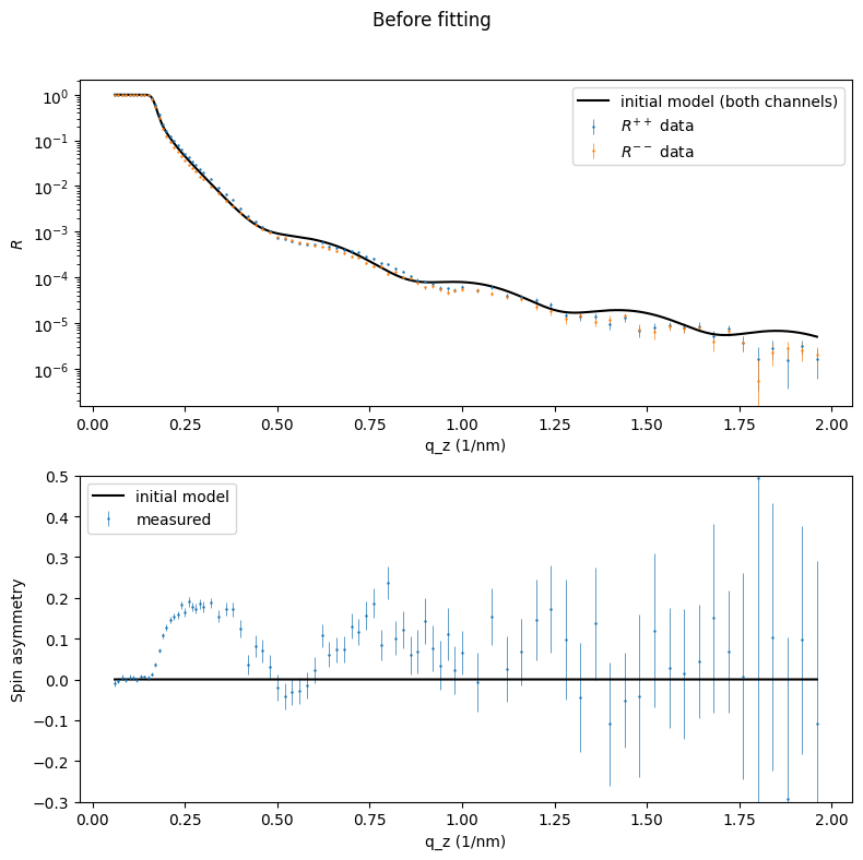
The spin asymmetry S = (R++ - R--)/(R++ + R--) is a derived diagnostic:
it is plotted, but not fitted separately. The initial model has zero
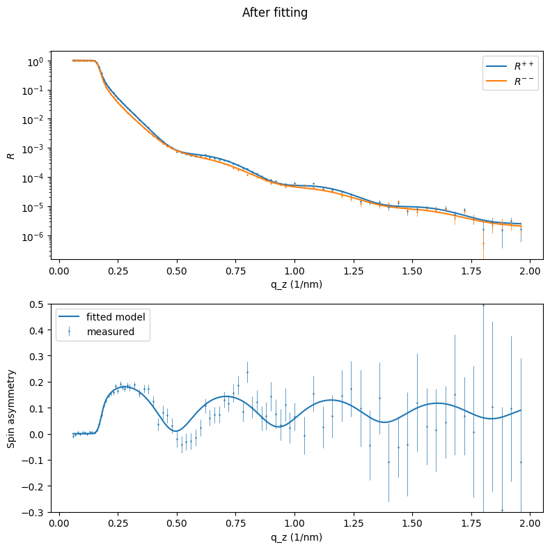
magnetic SLD and therefore no intrinsic spin contrast; the fit turns the
magnetization on. The companion example SpinAsymmetry simulates the fitted
model.
"""
import os
from pathlib import Path
import numpy as np
import bornagain as ba
ba.require_versions("bornagain>=25,<26")
from bornagain import nm, R3
import lmfit
MAO_SLD = (5.377e-06, 0) # SLD in Angstrom^-2
# Magnetic SLD in Angstrom^-2 per magnetization in A/m.
MAGNETIC_SLD_PER_MAGNETIZATION = 2.910429812376859e-12
def total_q_resolution(q_axis, dq_pointwise, sample_broadening):
"""
Combines pointwise instrument resolution with sample broadening.
The pointwise dQ is a standard deviation in 1/nm. The sample broadening is
an angular FWHM in degrees and is added linearly to the reconstructed
instrument angular FWHM, as in Refl1D. The wavelength and its resolution
are fixed by the MAFO experiment.
"""
wavelength = 0.475*nm
wavelength_resolution = 0.003*nm
fwhm_scale = np.sqrt(8*np.log(2))
theta = np.arcsin(q_axis*wavelength/(4*np.pi))
dq_spectral = q_axis*wavelength_resolution/wavelength
dq_angular = np.sqrt(dq_pointwise**2 - dq_spectral**2)
angular_fwhm = (
dq_angular*wavelength*fwhm_scale/(4*np.pi*np.cos(theta)))
angular_fwhm += np.deg2rad(sample_broadening)
dq_angular_broadened = (
(4*np.pi/wavelength)*np.cos(theta)*angular_fwhm/fwhm_scale)
return np.hypot(dq_spectral, dq_angular_broadened)
def get_sample(parameters):
"""
Magnesium aluminum ferrite (MAFO, from Mg-Al-Fe-O; MgAl0.5Fe1.5O4)
layer on a magnesium aluminate (MAO, MgAl2O4) substrate.
"""
magnetic_sld = parameters["mafo_magnetic_sld"]*1e-6
magnetization = R3(0, magnetic_sld/MAGNETIC_SLD_PER_MAGNETIZATION, 0)
vacuum = ba.Vacuum()
film_color = (0.45, 0.32, 0.80)
film_sld = parameters["mafo_sld"]*1e-6
film_material = ba.SLDMaterial(
"MgAl0.5Fe1.5O4", film_color, film_sld, 0, magnetization)
substrate_color = (0.28, 0.57, 0.82)
substrate_material = ba.SLDMaterial("MgAl2O4", substrate_color, *MAO_SLD)
film_autocorr = ba.SelfAffineFractalModel(
parameters["mafo_roughness"]*nm, 0.7, 25*nm)
substrate_autocorr = ba.SelfAffineFractalModel(
parameters["mao_roughness"]*nm, 0.7, 25*nm)
transient = ba.TanhTransient()
film_roughness = ba.Roughness(film_autocorr, transient)
substrate_roughness = ba.Roughness(substrate_autocorr, transient)
ambient_layer = ba.Layer(vacuum)
film_layer = ba.Layer(
film_material, parameters["mafo_thickness"]*nm, film_roughness)
substrate_layer = ba.Layer(substrate_material, substrate_roughness)
sample = ba.Sample()
sample.addLayer(ambient_layer)
sample.addLayer(film_layer)
sample.addLayer(substrate_layer)
return sample
def get_simulation(q_axis, q_resolution, parameters, spin_sign):
"""
Polarized specular simulation of one non-spin-flip channel.
q_axis and q_resolution contain one value per point, both in 1/nm.
spin_sign is +1 for the ++ channel, -1 for the -- channel.
"""
resolution_profile = ba.DistributionGaussian(0., 1., 25, 4.)
scan = ba.QzScan(q_axis)
scan.setOffset(parameters["q_offset"]/nm)
q_resolution = total_q_resolution(
q_axis, q_resolution, parameters["sample_broadening"])
scan.setVectorResolution(resolution_profile, q_resolution)
channel = R3(0, spin_sign, 0)
scan.setPolarization(channel)
scan.setAnalyzer(channel)
return ba.SpecularSimulation(scan, get_sample(parameters))
def load_data(filename):
"""
Reads dimensionless reflectivity, its uncertainty, and q resolution.
Interprets q and its pointwise standard deviation as 1/nm.
"""
# Data files are next to this script.
data_dir = Path(__file__).resolve().parent
filepath = data_dir / filename
q, reflectivity, uncertainty, q_resolution = ba.read_columns(
filepath, usecols=(0, 1, 2, 3))
return q/nm, reflectivity, uncertainty, q_resolution/nm
def qz_datafield(q, values, errors=()):
"""
Wraps dimensionless values and errors on a q_z axis given in 1/nm.
"""
return ba.Datafield(ba.Frame(ba.ListScan("q_z (1/nm)", list(q))),
np.asarray(values, dtype=float).tolist(),
np.asarray(errors, dtype=float).tolist())
def spin_asymmetry(r_pp, r_mm):
"""
Spin asymmetry S = (R++ - R--)/(R++ + R--); NaN where undefined.
"""
denominator = r_pp + r_mm
with np.errstate(divide='ignore', invalid='ignore'):
return np.where(denominator != 0, (r_pp - r_mm)/denominator, np.nan)
def spin_asymmetry_error(r_pp, r_mm, sigma_pp, sigma_mm):
"""
Uncertainty of the spin asymmetry, assuming independent channels.
"""
denominator = (r_pp + r_mm)**2
with np.errstate(divide='ignore', invalid='ignore'):
return np.where(denominator != 0,
2*np.sqrt(r_mm**2*sigma_pp**2
+ r_pp**2*sigma_mm**2)/denominator,
np.nan)
if __name__ == '__main__':
q_pp, r_pp, sigma_pp, q_res_pp = load_data("MAFO_Saturated_pp.tab")
q_mm, r_mm, sigma_mm, q_res_mm = load_data("MAFO_Saturated_mm.tab")
if not np.array_equal(q_pp, q_mm):
raise ValueError(
"Spin asymmetry requires both channels on the same q grid")
qz_data = q_pp
def residuals(fit_parameters):
"""
Concatenated sigma-weighted residuals of both channels,
so that their sum of squares is the chi-square objective.
"""
values = fit_parameters.valuesdict()
sim_pp = get_simulation(qz_data, q_res_pp, values, +1).simulate()
sim_mm = get_simulation(qz_data, q_res_mm, values, -1).simulate()
return np.concatenate([
(r_pp - sim_pp.intensities())/sigma_pp,
(r_mm - sim_mm.intensities())/sigma_mm
])
parameters = lmfit.Parameters()
parameters.add("sample_broadening", value=0.026, min=0, max=0.1) # deg
parameters.add("q_offset", value=0, min=-0.002, max=0.002) # (1/nm)
parameters.add("mafo_sld", value=6.3649, min=2, max=7) # (1e-6 Å⁻²)
parameters.add("mafo_magnetic_sld", value=0, min=0, max=2) # (1e-6 Å⁻²)
parameters.add("mafo_thickness", value=15, min=6, max=18) # (nm)
parameters.add("mao_roughness", value=0.1, min=0, max=1.2) # (nm)
parameters.add("mafo_roughness", value=0.1, min=0, max=1.2) # (nm)
initial_parameters = parameters.valuesdict()
fit_result = lmfit.minimize(
    residuals, parameters, method="leastsq",
    iter_cb=ba.Printer(every_nth=10))
print(lmfit.fit_report(fit_result))
fitted_parameters = fit_result.params.valuesdict()
ba.showSample3D(get_sample(fitted_parameters), sample_size=120*nm, seed=0)
# Evaluate smooth model curves on a denser q grid than the measured data.
qmin, qmax = 0.05997/nm, 1.96/nm
scan_size = 1500
qz_plot = np.linspace(qmin, qmax, scan_size)
q_res_plot_pp = np.interp(qz_plot, q_pp, q_res_pp)
q_res_plot_mm = np.interp(qz_plot, q_mm, q_res_mm)
# Both initial channels coincide because the magnetic SLD is zero.
initial_result = get_simulation(
qz_plot, q_res_plot_pp, initial_parameters, +1).simulate()
fitted_result_pp = get_simulation(
qz_plot, q_res_plot_pp, fitted_parameters, +1).simulate()
fitted_result_mm = get_simulation(
qz_plot, q_res_plot_mm, fitted_parameters, -1).simulate()
initial_intensity = initial_result.intensities()
initial_sa = spin_asymmetry(initial_intensity, initial_intensity)
fitted_sa = spin_asymmetry(fitted_result_pp.intensities(),
fitted_result_mm.intensities())
measured_sa = spin_asymmetry(r_pp, r_mm)
measured_sa_error = spin_asymmetry_error(r_pp, r_mm, sigma_pp, sigma_mm)
measured_result_pp = qz_datafield(qz_data, r_pp, sigma_pp)
measured_result_mm = qz_datafield(qz_data, r_mm, sigma_mm)
measured_sa_result = qz_datafield(qz_data, measured_sa, measured_sa_error)
initial_sa_result = qz_datafield(qz_plot, initial_sa)
fitted_sa_result = qz_datafield(qz_plot, fitted_sa)
# Plot the measured data and initial model before fitting.
initial_figure, (ax_initial_r, ax_initial_sa) = ba.plt.subplots(
2, 1, figsize=(8, 8), layout="constrained")
initial_figure.suptitle("Before fitting")
ba.plot_specular_curves(
[("$R^{++}$ data", measured_result_pp, None),
("$R^{--}$ data", measured_result_mm, None)],
ax=ax_initial_r, ylabel="$R$")
ba.plot_specular_curves(
[("initial model (both channels)", None, initial_result)],
ax=ax_initial_r, ylabel="$R$", color='black')
ax_initial_r.legend()
ba.plot_specular_curves(
[("measured", measured_sa_result, None)],
ax=ax_initial_sa, yscale='linear', ylim=(-0.3, 0.5),
ylabel="Spin asymmetry", color='C0')
ba.plot_specular_curves(
[("initial model", None, initial_sa_result)],
ax=ax_initial_sa, yscale='linear', ylim=(-0.3, 0.5),
ylabel="Spin asymmetry", color='black')
ax_initial_sa.legend()
# Plot the measured data and fitted model after fitting.
fitted_figure, (ax_fitted_r, ax_fitted_sa) = ba.plt.subplots(
2, 1, figsize=(8, 8), layout="constrained")
fitted_figure.suptitle("After fitting")
ba.plot_specular_curves(
[("$R^{++}$", measured_result_pp, fitted_result_pp),
("$R^{--}$", measured_result_mm, fitted_result_mm)],
ax=ax_fitted_r, ylabel="$R$")
ax_fitted_r.legend()
ba.plot_specular_curves(
[("measured", measured_sa_result, None)],
ax=ax_fitted_sa, yscale='linear', ylim=(-0.3, 0.5),
ylabel="Spin asymmetry", color='C0')
ba.plot_specular_curves(
[("fitted model", None, fitted_sa_result)],
ax=ax_fitted_sa, yscale='linear', ylim=(-0.3, 0.5),
ylabel="Spin asymmetry", color='C0')
ax_fitted_sa.legend()
ba.plt.show()
|