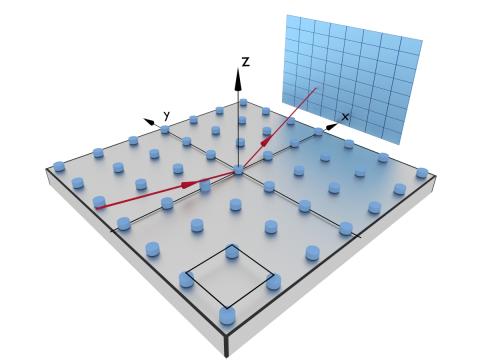
We consider a 2D Bravais lattice that is specified by lattice constants $a$ and $b$, by the angle $\alpha$ between the lattice vectors $\mathbf{a}$ and $\mathbf{b}$, and by the angle $\xi$ between $\mathbf{a}$ and the $x$ axis of the instrument frame.

The structure for an infinite 2D lattice is created from a particle and a lattice object:
lattice = ba.BasicLattice2D(length_a, length_b, alpha, xi)
structure = ba.Crystal2D(particle, lattice)
To account for finite-size effects, and to give the simulated Bragg peaks a finite width, attach a peak profile as described below.
The finite 2D lattice model is computed by explicit summation over contributions from all unit cells. The lattice is constructed by one of the following:
ba.BasicLattice2D(length_a, length_b, alpha, xi)
ba.SquareLattice2D(length, xi)
ba.HexagonalLattice2D(length, xi)
Then the finite structure is constructed by
structure = ba.FiniteCrystal2D(particle, lattice, size_a, size_b)
where the arguments $\textrm{size}_a$ and $\textrm{size}_b$ are the crystal sizes in lattice directions $\mathbf{a}$ and $\mathbf{b}$. Each size is rounded to the nearest integer number of unit cells; the crystal is a parallelogram spanned by the two lattice vectors.
The decay function accounts for the finite size of the sample, the crystalline domain, or the scattering volume. It contributes a multiplicative factor $h(\mathbf{r})$ to the correlation function in real space that lets it decay for $r$.
Equivalently, its Fourier transform $H(\mathbf{q})$ is convolved with the structure factor of the ideal, infinite lattice,
$$S_0(\mathbf{q}) = \rho \sum_i c_i \delta(\mathbf{q} - \mathbf{q}_i),$$
where the sum runs over reciprocal lattice points, resulting in
$$S(\mathbf{q}) = \rho \sum_i c_i H(\mathbf{q} - \mathbf{q}_i).$$
That is, each Bragg peak gets the same smooth profile $H(\mathbf{q})$ instead of the infinitely sharp delta function.

Decay functions for the one-dimensional case are explained in the grating section. Decay functions for two-dimensional lattices work similarly, but require two length parameters and an orientation. The lengths $\omega_x$ and $\omega_y$ refer to the principal axes of an ellipsis that is rotated by an angle $\gamma$ with respect to the coordinate axes $x$, $y$.
BornAgain supports three two-dimensional decay functions:
ba.Profile2DCauchy(omega_x, omega_y, gamma)
ba.Profile2DGauss(omega_x, omega_y, gamma)
ba.Profile2DVoigt(omega_x, omega_y, gamma, eta)
The Cauchy distribution is in physics better known as the Lorentzian profile.
The Voigt distribution is computed as the true convolution of a Gaussian and a
Lorentzian, using our numeric library
libcerf. The dimensionless
parameter eta=$\eta$ may take values between 0 (Lorentian) and 1 (Gaussian).
Decay lengths should be much larger than the lattice constants. Otherwise the model becomes physically questionable, and computation times increase a lot. Typical values for meaningful decay lengths are in the micrometer range (≥ 1000 nm).
The decay function is attached to a lattice structure by the
setDecayFunction method:
lattice = ba.BasicLattice2D(20*nm, 20*nm, 120*deg, 0)
structure = ba.Crystal2D(particle, lattice)
profile = ba.Profile2DCauchy(1000*nm, 1000*nm, 0*deg)
structure.setDecayFunction(profile)
The particle density is determined from the 2D lattice parameters. There is no
separate particle-density setting for Crystal2D or FiniteCrystal2D.