 BornAgain
≻ git-develop
≻ Documentation ≻ Reference ≻ Data types ≻ Class Datafield ≻ Axis coordinates and transformations
BornAgain
≻ git-develop
≻ Documentation ≻ Reference ≻ Data types ≻ Class Datafield ≻ Axis coordinates and transformations
BornAgain
≻ git-develop
≻ Documentation ≻ Reference ≻ Data types ≻ Class Datafield ≻ Axis coordinates and transformations
BornAgain
≻ git-develop
≻ Documentation ≻ Reference ≻ Data types ≻ Class Datafield ≻ Axis coordinates and transformations
A scattering simulation with a SphericalDetector returns exit-angle axes
phi_f (rad) and alpha_f (rad). Plots display radian axes in degrees. To
access the converted coordinates directly:
degree_result = angular_result.plottableField()
phi_f_degrees = degree_result.xCenters()
alpha_f_degrees = degree_result.yCenters()
Use the beam wavelength in nm and incident grazing angle in rad:
transformation = ba.FrameTrafo.ScatteringToQ(wavelength, alpha_i)
q_result = transformation.transformedDatafield(angular_result)
For a nonzero incident azimuth, pass phi_i as the third argument. The
transformation follows
$$ q_y = \frac{2\pi}{\lambda} \left(\sin\varphi_\mathrm{f}-\sin\varphi_\mathrm{i}\right), \qquad q_z = \frac{2\pi}{\lambda} \left(\sin\alpha_\mathrm{f}+\sin\alpha_\mathrm{i}\right). $$
The result has axes q_y (1/nm) and q_z (1/nm). Intensity values remain in
the same bin order: ScatteringToQ changes the axes but does not rebin or
interpolate the map. Its two independent equidistant q axes are a small-angle
approximation.
The input must have the angular axis labels shown above. There is no inverse q-to-angle transformation, and offspec results are not supported.
For a specular simulation, choose angular or q coordinates when creating the scan:
angular_scan = ba.AlphaScan(n, alpha_min, alpha_max)
q_scan = ba.QzScan(n, q_z_min, q_z_max)
To exchange both axes and transpose the values:
transposed_result = ba.FrameTrafo.Transpose(q_result)
For custom axes, construct a new frame and attach the corresponding values:
custom_frame = ba.Frame(
    ba.ListScan("x (nm)", x_coordinates.tolist()),
    ba.ListScan("y (nm)", y_coordinates.tolist()))
custom_result = ba.Datafield(custom_frame, transformed_values.ravel().tolist())
This constructor does not transform or interpolate values. For a reciprocal-space to real-space transformation, see Fourier transform example.
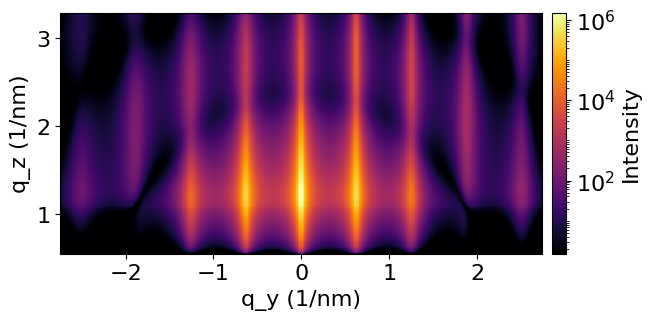
Scattering intensity
This functionality was provided in completely different ways in BornAgain <=21. The present solution has been introduced in BornAgain 24.