 BornAgain
≻ git-develop
≻ Documentation ≻ Reference ≻ Fitting ≻ Examples ≻ Reflectometry: Fit Pt layer
BornAgain
≻ git-develop
≻ Documentation ≻ Reference ≻ Fitting ≻ Examples ≻ Reflectometry: Fit Pt layer
BornAgain
≻ git-develop
≻ Documentation ≻ Reference ≻ Fitting ≻ Examples ≻ Reflectometry: Fit Pt layer
BornAgain
≻ git-develop
≻ Documentation ≻ Reference ≻ Fitting ≻ Examples ≻ Reflectometry: Fit Pt layer
In this example, we want to demonstrate how to fit experimental reflectivity data that was obtained by a time-of-flight experiment with unpolarized neutrons. Experimental data is available for a sample of a roughly 50 nm thick platinum layer on top of a silicon substrate that is published in this repository.
The mesaurements were made by Timothy Charlton, Haile Ambaye and Michael Fitzsimmons (ORNL) on a sample provided by Eric Fullerton (UCSD).
The fourth data column is the full width of a logarithmic $q$ bin. The
source notebook
writes it as the difference between adjacent bin edges for bins with
$\Delta q/q=0.01$. It is not a Gaussian instrument resolution and is
therefore not passed to QzScan.setVectorResolution.
We describe the above experiment by a three-layer model, where as usual the top layer is the vacuum and the substrate layer is the silicon substrate. On top of the silicon substrate, we place the platinum layer. The materials of both layers are described by their SLD, where we use literature values for both silicon as well as platinum and keep them constant throughout the fitting procedure.
The fit uses the following six lmfit parameters:
Dimensionless beam-intensity scale: intensity
We explicitly fit the beam intensity, in order to compensate for possible experimental errors and to circumvent problems with the rather large variance in the reflectivity data at low $Q$-values.
Roughness on top of the Pt layer in nm: r_pt
Roughness on top of the Si substrate in nm: r_si
Thickness of the Pt layer in nm: t_pt
The absolute Gaussian $Q$-resolution: q_resolution, in nm$^{-1}$
A $Q$-offset in nm$^{-1}$: q_offset
This global offset is introduced to account for uncertainties in the angle at which the measurement is performed.
Due to saturation of the detector it is possible that the intensity at low $Q$-values (i.e. at high count rates) is underestimated. Furthermore, there is a rather large variance in the data that also leads to a rather bad fit in this region. Therefore, we neglect the data in the low $Q$-region by choosing a cutoff at $Q_{\text{min}} = $ 0.18 nm$^{-1}$. This value is selected by hand after performing several fits and visually selecting a good result.
The offset is assigned directly to the scan before performing a simulation:
scan = ba.QzScan(q_axis)
scan.setOffset(P["q_offset"])
The example uses starting values sufficiently close to the measured sample. Run it with:
python3 Pt_layer_fit.py
This performs a simulation with the initial parameters. The initial model is shown in the left panel of the generated comparison below.
Immediately afterwards the fit is performed.
The script then performs the fit and compares both states:
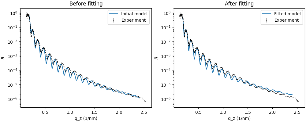
Measured data with the initial and fitted models
|
|