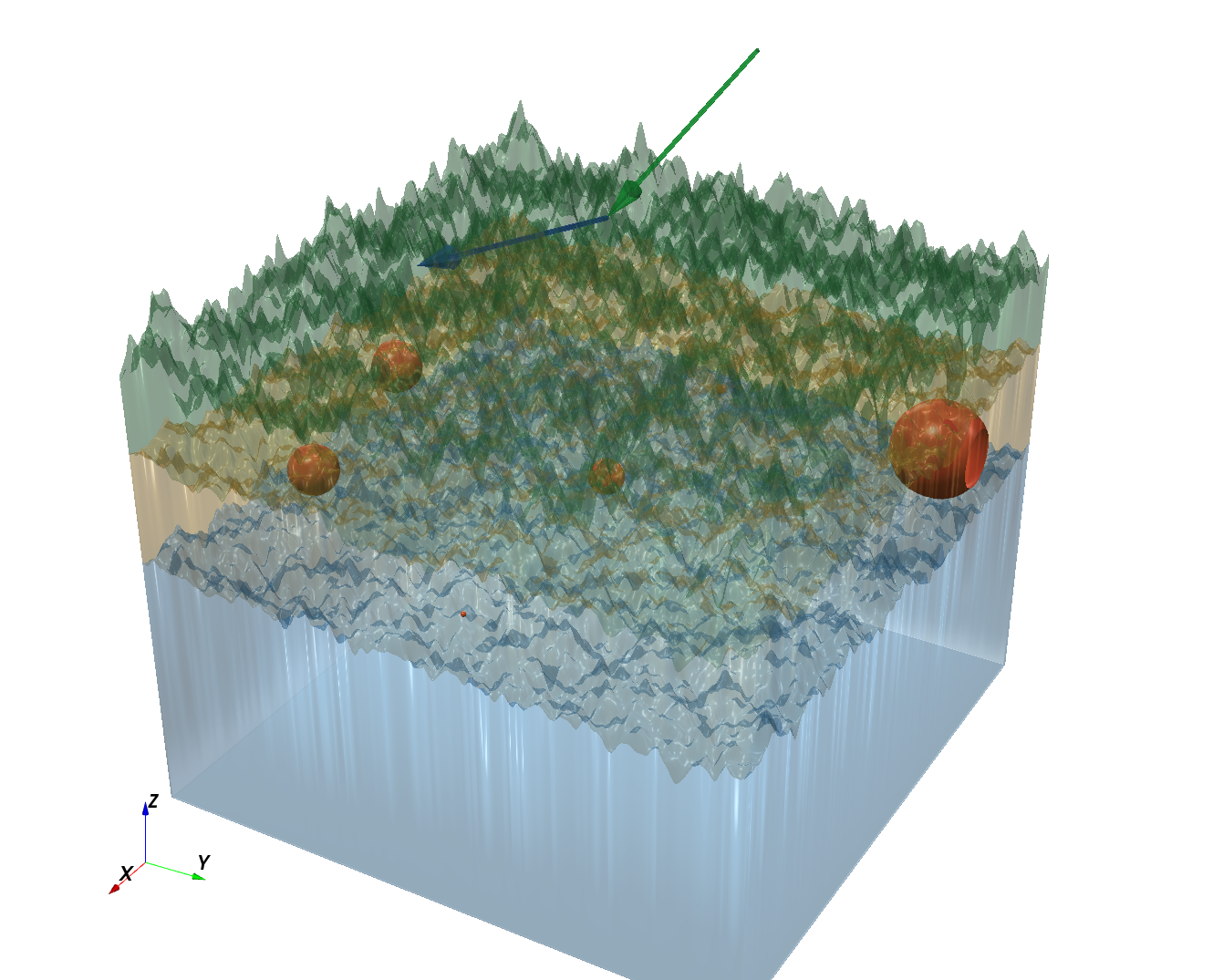
1
  2
  3
  4
  5
  6
  7
  8
  9
 10
 11
 12
 13
 14
 15
 16
 17
 18
 19
 20
 21
 22
 23
 24
 25
 26
 27
 28
 29
 30
 31
 32
 33
 34
 35
 36
 37
 38
 39
 40
 41
 42
 43
 44
 45
 46
 47
 48
 49
 50
 51
 52
 53
 54
 55
 56
 57
 58
 59
 60
 61
 62
 63
 64
 65
 66
 67
 68
 69
 70
 71
 72
 73
 74
 75
 76
 77
 78
 79
 80
 81
 82
 83
 84
 85
 86
 87
 88
 89
 90
 91
 92
 93
 94
 95
 96
 97
 98
 99
100
101
102
103
104
105
106
107
108
109
110
111
112
113
114
115
116
117
118
119
120
121
122
123
124
125
126
127
128
129
130
131
132
133
134
135
136
137
138
139
140
141
142
143
144
145
146
147
148
149
150
151
152
153
154
155
156
157
158
159
160
161
162
163
164
165
166
167
168
169
170
171
172
173
174
175
176
177
178
179
180
181
182
183
184
185
186
187
188
189
190
191
192
193
194
195
196
197
198
199
200
201
202
203
204
205
206
207
208
209
210
211
212
213
214
215
216
217
218
219
220
221
222
223
224
225
226
227
228
229
230
231
232
233
234
235
236
237
238
239
240
241
242
243
244
245
246
247
248
249
250
251
252
253
254
255
256
257
258
259
260
261
262
263
264
265
266
267
268
269
270
271
272
273
274
275
276
277
278
279
280
281
282
|
#!/usr/bin/env python3
# /// script
# requires-python = ">=3.10"
# dependencies = ["bornagain>=25,<26", "fabio", "lmfit"]
# ///
"""
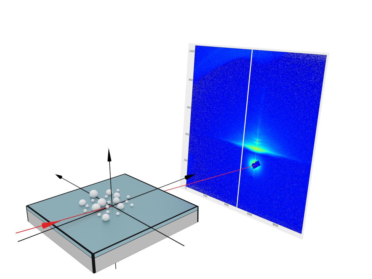
Fitting experimental data: spherical nanoparticles with size distribution
in a four-layer system (experiment at GALAXI).

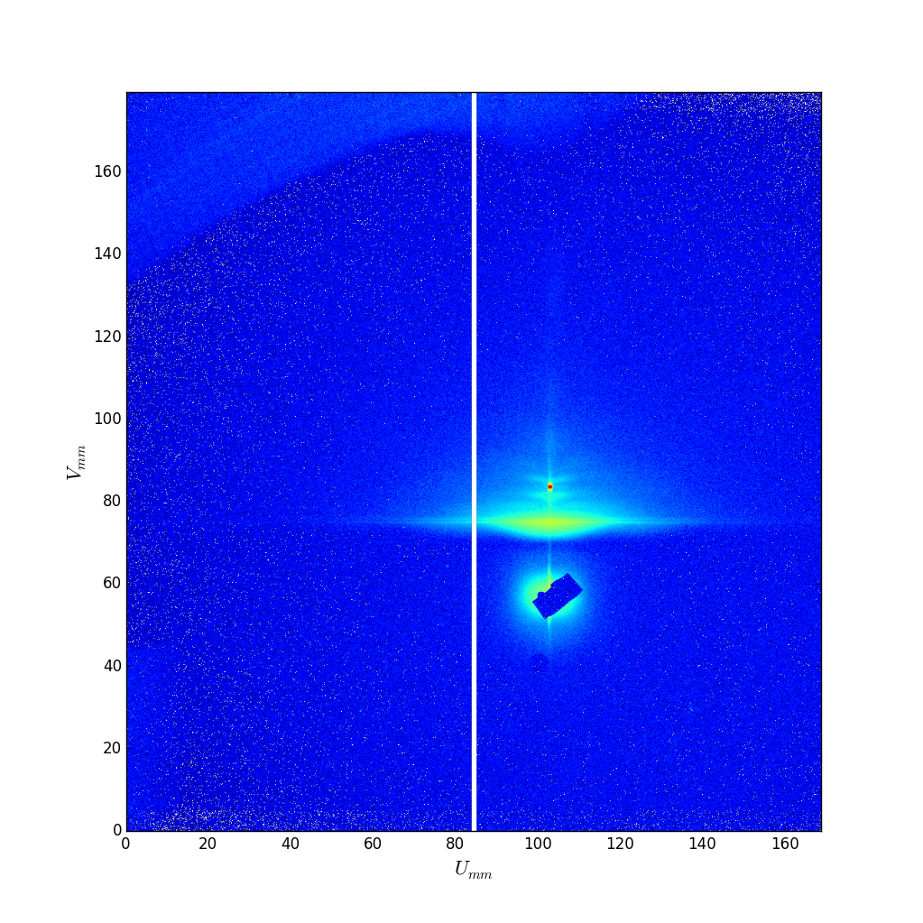
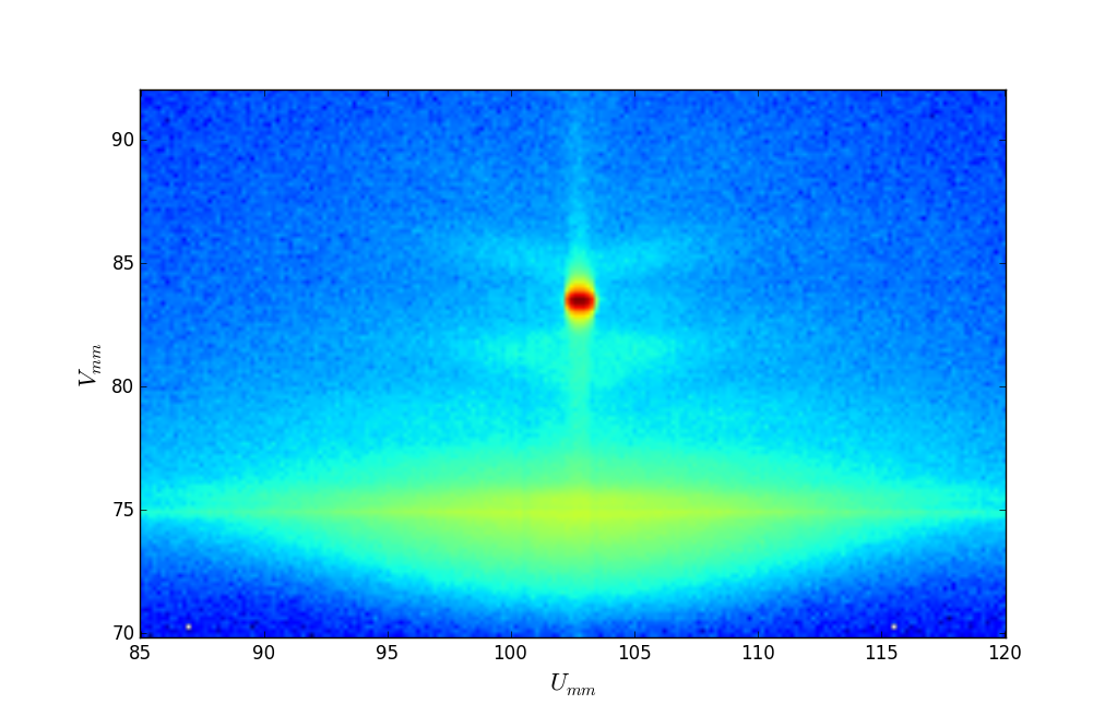
Demonstrates how to load a detector image with fabio, anchor the
detector geometry to the direct-beam position, crop the data and
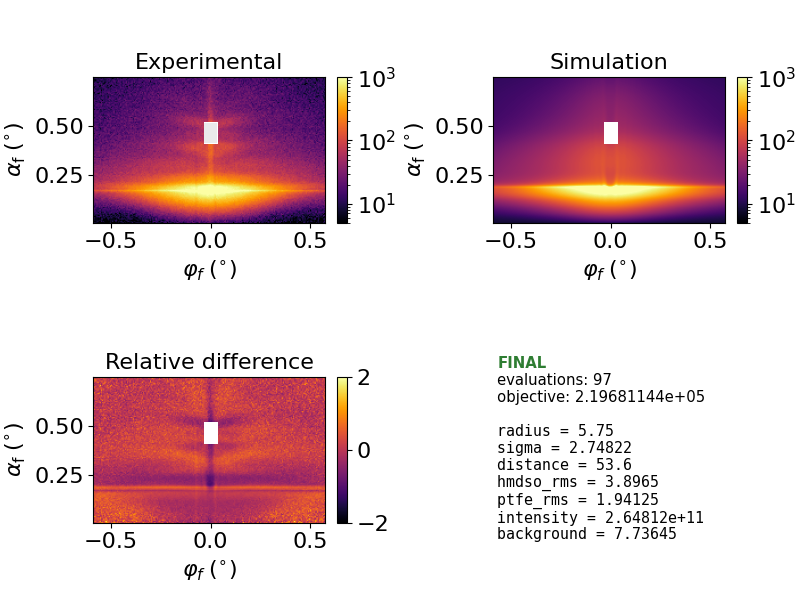
detector to the fit window, and compare a polydisperse sample model
to the data by fitting the particle-size distribution width, interface
roughnesses, intensity normalization, and constant background.
"""
from pathlib import Path
import bornagain as ba
ba.require_versions("bornagain>=25,<26")
from bornagain import R3, angstrom, deg, nm
import lmfit
import numpy as np


def get_mixture(ag_mat, radius, sigma, hmdso_thickness):
    """
    Creates a log-normal mixture of Ag spheres that fit in the HMDSO layer.
    """
    nsizes = 20
    r_min = radius*np.exp(-2*sigma)
    r_max = min(radius*np.exp(2*sigma), hmdso_thickness/2)
    radii = np.linspace(r_min, r_max, nsizes)
    weights = np.exp(-np.log(radii/radius)**2/(2*sigma**2))/radii
    mixture = ba.Mixture()  # normalizes the weights
    for r, w in zip(radii, weights):
        sphere = ba.Particle(ag_mat, ba.Sphere(r))
        sphere.translate(R3(0, 0, -hmdso_thickness))
        mixture.addParticle(sphere, w)
    return mixture


def get_sample(P):
    """
    Creates the layered GALAXI sample for the fit parameters P.
    """
    radius = P["radius"]*nm
    sigma = P["sigma"]
    distance = P["distance"]*nm
    disorder = 10.5*nm
    kappa = 17.5
    ptfe_thickness = 22.1*nm
    hmdso_thickness = 18.5*nm

    # defining materials
    si_color = (0.30, 0.62, 0.86)
    ag_color = (0.86, 0.24, 0.18)
    ptfe_color = (0.93, 0.72, 0.25)
    hmdso_color = (0.25, 0.65, 0.35)

    si_mat = ba.RefractiveMaterial("Si", si_color, 5.7816e-6, 1.0229e-7)
    ag_mat = ba.RefractiveMaterial("Ag", ag_color, 2.2475e-5, 1.6152e-6)
    ptfe_mat = ba.RefractiveMaterial("PTFE", ptfe_color, 5.20509e-6, 1.9694e-8)
    hmdso_mat = ba.RefractiveMaterial("HMDSO", hmdso_color, 2.0888e-6, 1.3261e-8)

    # collection of particles with size distribution
    mixture = get_mixture(ag_mat, radius, sigma, hmdso_thickness)

    # interference function
    layout = ba.RadialParacrystal(mixture, distance, 1e6*nm)
    layout.setKappa(kappa)
    layout.setDomainSize(2e4*nm)
    profile = ba.Profile1DGauss(disorder)
    layout.setProbabilityDistribution(profile)

    vertical_correlation_depth = 100*nm
    hmdso_roughness_rms = P["hmdso_rms"]*nm
    ptfe_roughness_rms = P["ptfe_rms"]*nm
    # The unmeasured PTFE/Si interface uses the PTFE roughness scale.
    substrate_roughness_rms = ptfe_roughness_rms
    roughness_hurst = 0.3
    lateral_correlation_length = 5*nm

    # Self-affine roughness on all interfaces. The upper two interfaces
    # are vertically correlated with the interface below.
    hmdso_autocorr = ba.SelfAffineFractalModel(
        hmdso_roughness_rms, roughness_hurst,
        lateral_correlation_length)
    ptfe_autocorr = ba.SelfAffineFractalModel(
        ptfe_roughness_rms, roughness_hurst,
        lateral_correlation_length)
    substrate_autocorr = ba.SelfAffineFractalModel(
        substrate_roughness_rms, roughness_hurst,
        lateral_correlation_length)
    transient = ba.TanhTransient()
    crosscorr = ba.CommonDepthCrosscorrelation(vertical_correlation_depth)
    hmdso_roughness = ba.Roughness(
        hmdso_autocorr, transient, crosscorr)
    ptfe_roughness = ba.Roughness(
        ptfe_autocorr, transient, crosscorr)
    substrate_roughness = ba.Roughness(substrate_autocorr, transient)

    # layers
    vacuum_layer = ba.Layer(ba.Vacuum())
    hmdso_layer = ba.Layer(hmdso_mat, hmdso_thickness, hmdso_roughness)
    hmdso_layer.deposit2D(layout)
    ptfe_layer = ba.Layer(ptfe_mat, ptfe_thickness, ptfe_roughness)
    substrate_layer = ba.Layer(si_mat, substrate_roughness)

    # assembling sample
    sample = ba.Sample()
    sample.addLayer(vacuum_layer)
    sample.addLayer(hmdso_layer)
    sample.addLayer(ptfe_layer)
    sample.addLayer(substrate_layer)

    return sample


def detector_angle_range(pixel_centers, pixel_size, beam_position,
                         detector_distance, beam_center_angle):
    """
    Returns the angular range covered by the given flat-detector pixels.

    beam_center_angle is the physical angle at the direct-beam position.
    """
    def detector_angle(position):
        return (np.arctan2(position - beam_position, detector_distance)
                + beam_center_angle)

    lower_edge = pixel_centers[0] - pixel_size/2
    upper_edge = pixel_centers[-1] + pixel_size/2
    return detector_angle(lower_edge), detector_angle(upper_edge)


def get_simulation(P, detector, alpha_i):
    """
    Creates a GISAS simulation for the fit parameters P.
    """
    wavelength = 1.34*angstrom
    beam = ba.Beam(P["intensity"], wavelength, alpha_i)
    sample = get_sample(P)
    simulation = ba.ScatteringSimulation(beam, sample, detector)
    simulation.setBackground(ba.ConstantBackground(P["background"]))
    return simulation


def load_data(filename, window_mask):
    """
    Loads, orients, and crops the experimental detector image.
    """
    import fabio
    # Data files are next to this script.
    data_dir = Path(__file__).resolve().parent
    filepath = data_dir / filename
    raw_data = fabio.open(filepath).data.astype(float)
    # Fabio puts row 0 at the top; BornAgain expects the lowest angle first.
    data = np.flipud(raw_data)
    return ba.crop_by_mask(data, window_mask)


def get_plotters(exp_data):
    """
    Creates the fit-progress plotters.
    """
    norm = ba.intensity_norm(exp_data, zmin=5, zmax=1e3)

    experiment_plotter = ba.FitPlotter(
        ba.plot_masked_experimental,
        measured=exp_data,
        norm=norm,
        with_cb=True,
        title="Experimental",
    )

    simulation_plotter = ba.FitPlotter(
        ba.plot_heatmap,
        norm=norm,
        with_cb=True,
        title="Simulation",
    )

    difference_plotter = ba.FitPlotter(
        ba.plot_difference,
        measured=exp_data,
        with_cb=True,
        title="Relative difference",
    )

    return [
        experiment_plotter,
        simulation_plotter,
        difference_plotter,
    ]


if __name__ == '__main__':
    # Detector setup as given by the instrument responsible.
    full_nx = 981
    full_ny = 1043
    pixel_size = 0.172  # in mm
    detector_distance = 1730  # in mm
    beam_x_pixel_pos, beam_y_pixel_pos = 597.1, 323.4  # from lower left
    alpha_i = 0.463*deg

    # Pixel-center coordinates and fit window, in mm on the detector.
    x_pixels = (np.arange(full_nx) + 0.5)*pixel_size
    y_pixels = (np.arange(full_ny) + 0.5)*pixel_size
    x_grid, y_grid = np.meshgrid(x_pixels, y_pixels)
    inside_window = ((x_grid > 85) & (x_grid < 120)
                     & (y_grid > 70) & (y_grid < 92))
    window_mask = np.logical_not(inside_window)
    fit_x = ba.crop_by_mask(x_grid, window_mask)
    fit_y = ba.crop_by_mask(y_grid, window_mask)

    # Convert the selected pixel edges to the spherical-detector angles.
    beam_x_pos = beam_x_pixel_pos*pixel_size
    beam_y_pos = beam_y_pixel_pos*pixel_size
    phi_min, phi_max = detector_angle_range(
        fit_x[0, :], pixel_size, beam_x_pos, detector_distance, 0)
    alpha_min, alpha_max = detector_angle_range(
        fit_y[:, 0], pixel_size, beam_y_pos, detector_distance, -alpha_i)

    # Exclude the specular beam from the cropped detector.
    specular_beam_mask = ((fit_x > 101.9) & (fit_x < 103.7)
                          & (fit_y > 82.1) & (fit_y < 85.2))

    cropped_ny, cropped_nx = fit_x.shape
    detector = ba.SphericalDetector(
        cropped_nx, phi_min, phi_max,
        cropped_ny, alpha_min, alpha_max)
    detector.setMask(specular_beam_mask)

    data = load_data("galaxi_data.tif.gz", window_mask)
    # usable pixels: outside the specular beam, no detector gaps (-1)
    usable = (np.logical_not(specular_beam_mask)
              & np.isfinite(data) & (data >= 0))
    flat_exp_values = data[usable]
    display_data = np.where(usable, data, np.nan)
    exp_data = ba.Datafield(detector.frame(), display_data.ravel().tolist())

    # Fit progress display
    monitor = ba.FitMonitor(
        get_plotters(exp_data),
        ncols=2,
        show_best=True,
        max_fps=1,
        printer=ba.Printer(every_nth=10),
        live=True)

    def residuals(P):
        """
        Simulates, reports, and returns Poisson-weighted residuals.
        """
        p = P.valuesdict()
        sim_result = get_simulation(p, detector, alpha_i).simulate()
        flat_sim_values = sim_result.intensities()[usable]
        residuals = ((flat_exp_values - flat_sim_values)
                     / np.sqrt(np.maximum(1., flat_sim_values)))
        monitor.update(sim_result, P, residuals)
        return residuals

    P = lmfit.Parameters()
    # The mean particle radius and distance retain their reported values.
    P.add("radius", value=5.75, vary=False)  # (nm)
    P.add("sigma", value=0.4, min=0., max=3., vary=True)  # (dimensionless)
    P.add("distance", value=53.6, vary=False)  # (nm)
    # RMS roughnesses start from the values reported for the sample.
    P.add("hmdso_rms", value=1.1, min=0., max=5.)  # (nm)
    P.add("ptfe_rms", value=2.3, min=0., max=5.)  # (nm)
    # Effective normalization combines source flux and particle density.
    P.add("intensity", value=4e10, min=1e9, max=1e12)  # (a.u.)
    P.add("background", value=1., min=0., max=50.)  # (counts/pixel)

    result = lmfit.minimize(residuals, P, method="leastsq")

    finalP = result.params.valuesdict()
    # Recompute and report the simulation at the fitted parameters.
    residuals(result.params)
    # Render the just-reported evaluation as the final fit state.
    monitor.render_final(result.params)
    print(lmfit.fit_report(result))
    ba.showSample3D(get_sample(finalP), sample_size=120*nm, seed=228)
    ba.plt.show()
|