1
  2
  3
  4
  5
  6
  7
  8
  9
 10
 11
 12
 13
 14
 15
 16
 17
 18
 19
 20
 21
 22
 23
 24
 25
 26
 27
 28
 29
 30
 31
 32
 33
 34
 35
 36
 37
 38
 39
 40
 41
 42
 43
 44
 45
 46
 47
 48
 49
 50
 51
 52
 53
 54
 55
 56
 57
 58
 59
 60
 61
 62
 63
 64
 65
 66
 67
 68
 69
 70
 71
 72
 73
 74
 75
 76
 77
 78
 79
 80
 81
 82
 83
 84
 85
 86
 87
 88
 89
 90
 91
 92
 93
 94
 95
 96
 97
 98
 99
100
101
102
103
104
105
106
107
108
109
110
111
112
113
114
115
116
117
118
119
120
121
122
123
124
125
126
127
128
129
130
131
|
#!/usr/bin/env python3
# /// script
# requires-python = ">=3.10"
# dependencies = ["bornagain>=25,<26", "lmfit"]
# ///
"""
Basic GISAS 2D fitting example.
Fake experimental data are generated from a known sample model.
"""

import bornagain as ba
ba.require_versions("bornagain>=25,<26")
from bornagain import deg, nm, nm2
import lmfit
import numpy as np


def get_sample(P):
    """
    Dilute cylinders on a substrate, parameterized for GISAS fitting.
    """
    substrate_color = (0.28, 0.57, 0.82)
    particle_color = (0.86, 0.24, 0.18)

    substrate_mat = ba.RefractiveMaterial("Substrate", substrate_color, 6e-6, 2e-8)
    particle_mat = ba.RefractiveMaterial("Particle", particle_color, 6e-4, 2e-8)
    cylinder_ff = ba.Cylinder(P["cylinder_radius"], P["cylinder_height"])
    particle = ba.Particle(particle_mat, cylinder_ff)

    particle_layer = ba.Layer(ba.Vacuum())
    # Modest coverage keeps material averaging physical over the fit bounds.
    particle_layer.deposit2D(ba.Dilute2D(1e-3/nm2, particle))

    sample = ba.Sample()
    sample.addLayer(particle_layer)
    sample.addLayer(ba.Layer(substrate_mat))
    return sample


def get_simulation(P):
    """
    GISAS simulation with fitted beam intensity and background.
    """
    beam = ba.Beam(10**P["lg_intensity"], 0.1*nm, 0.2*deg)
    detector = ba.SphericalDetector(100, -1.5*deg, 1.5*deg, 100, 0, 3*deg)
    simulation = ba.ScatteringSimulation(beam, get_sample(P), detector)
    simulation.setBackground(ba.ConstantBackground(10**P["lg_background"]))
    return simulation


def get_plotters(exp_data):
    """
    Creates the fit-progress plotters.
    """
    norm = ba.intensity_norm(exp_data)

    experiment_plotter = ba.FitPlotter(
        ba.plot_experimental,
        measured=exp_data,
        norm=norm,
        with_cb=True,
        title="Experimental",
    )

    simulation_plotter = ba.FitPlotter(
        ba.plot_heatmap,
        norm=norm,
        with_cb=True,
        title="Simulation",
    )

    difference_plotter = ba.FitPlotter(
        ba.plot_difference,
        measured=exp_data,
        with_cb=True,
        title="Relative difference",
    )

    return [
        experiment_plotter,
        simulation_plotter,
        difference_plotter,
    ]


if __name__ == '__main__':
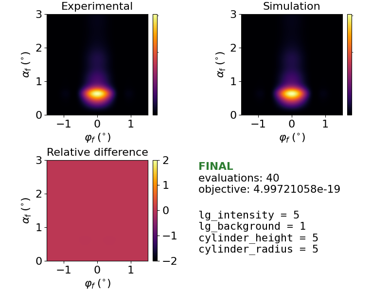
    fake_params = {
        "lg_intensity": 5,
        "lg_background": 1,
        "cylinder_height": 5.*nm,
        "cylinder_radius": 5.*nm,
    }
    exp_data = get_simulation(fake_params).simulate()
    flat_exp_values = exp_data.intensities().ravel()

    # Fit progress display
    monitor = ba.FitMonitor(
        get_plotters(exp_data),
        ncols=2,
        show_best=True,
        max_fps=1,
        printer=ba.Printer(every_nth=10),
        live=True)

    def residuals(P):
        """
        Simulates, reports, and returns the residual vector.
        """
        sim_result = get_simulation(P.valuesdict()).simulate()
        flat_sim_values = sim_result.intensities().ravel()
        residuals = flat_exp_values - flat_sim_values
        monitor.update(sim_result, P, residuals)
        return residuals

    P = lmfit.Parameters()
    P.add("lg_intensity", value=4.3, min=0, max=15)  # (dimensionless)
    P.add("lg_background", value=2.0, min=-2, max=10)  # (dimensionless)
    P.add("cylinder_height", value=8*nm, min=0.01*nm)
    P.add("cylinder_radius", value=3.5*nm, min=0.01*nm, max=8*nm)

    result = lmfit.minimize(residuals, P, method="leastsq")

    finalP = result.params.valuesdict()
    # Recompute and report the simulation at the fitted parameters.
    residuals(result.params)
    # Render the just-reported evaluation as the final fit state.
    monitor.render_final(result.params)
    print("Fit completed.")
    print(lmfit.fit_report(result))
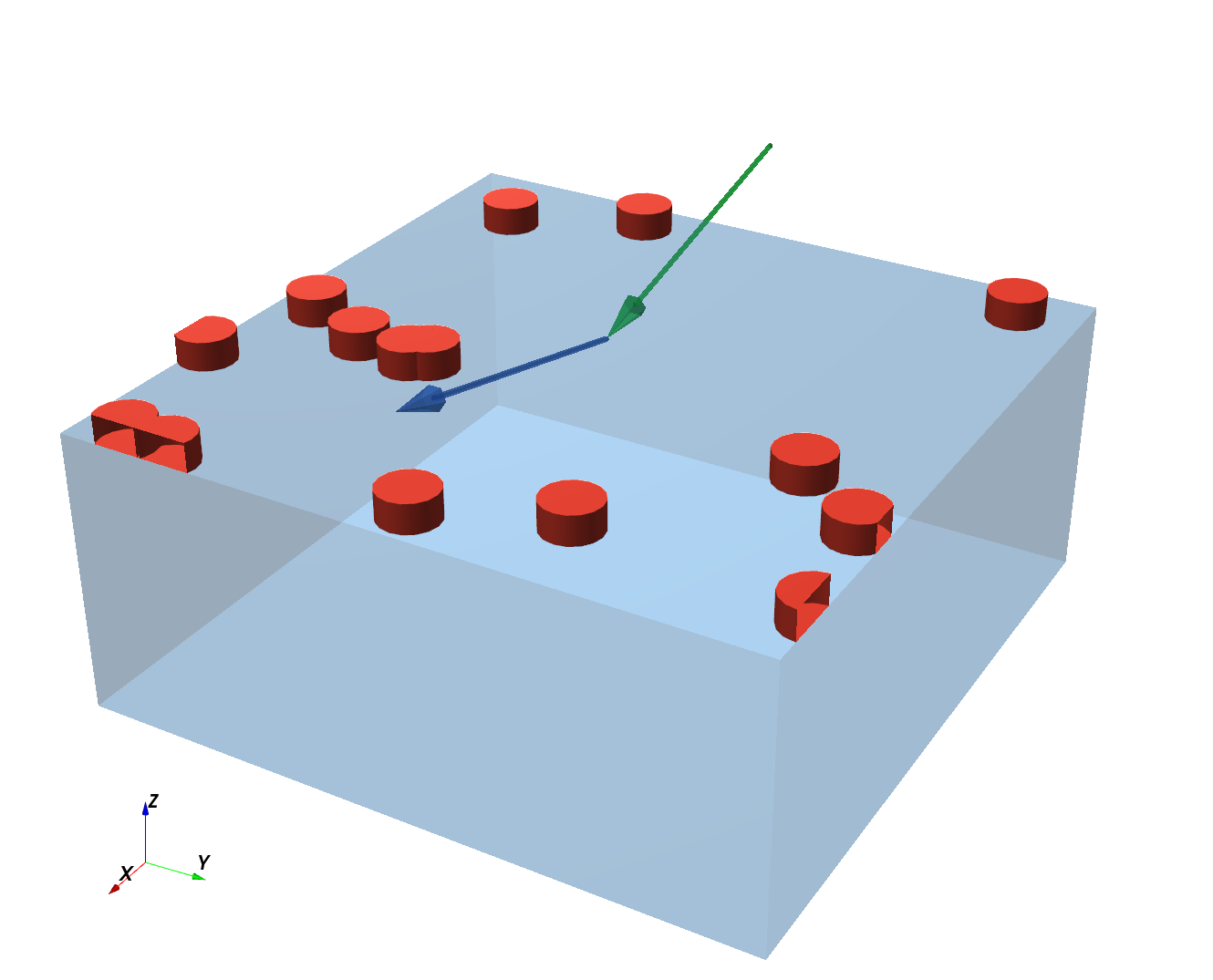
    ba.showSample3D(get_sample(finalP), sample_size=120*nm, seed=0)
    ba.plt.show()
|