1
 2
 3
 4
 5
 6
 7
 8
 9
10
11
12
13
14
15
16
17
18
19
20
21
22
23
24
25
26
27
28
29
30
31
32
33
34
35
36
37
38
39
40
41
42
43
44
45
46
47
48
49
50
51
52
53
54
55
56
57
58
59
60
61
62
63
64
65
66
67
68
69
70
71
72
73
74
75
76
77
78
79
80
81
82
83
84
85
|
#!/usr/bin/env python3
# /// script
# requires-python = ">=3.10"
# dependencies = ["bornagain>=25,<26"]
# ///
"""
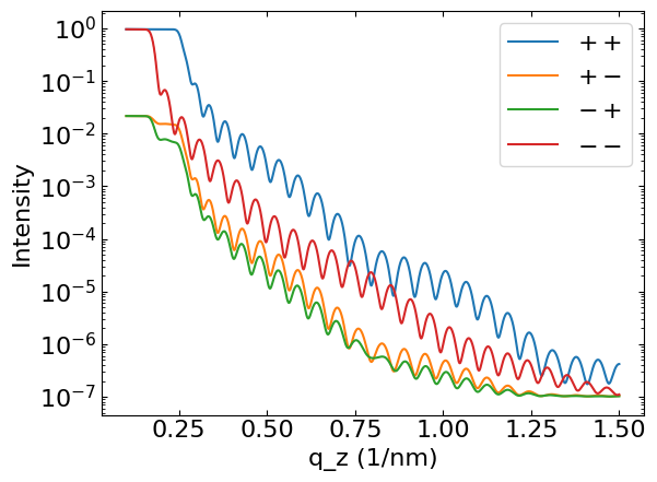
Realistic (imperfect) example for polarized reflectometry.
Sample contains a magnetic layer,
similar to Devishvili et al., Rev. Sci. Instrum. 84, 025112 (2013).
"""
import numpy as np
import bornagain as ba
ba.require_versions("bornagain>=25,<26")
from bornagain import nm, deg, R3
from math import sin, cos

def get_sample():
    # Materials
    Bmag = 1.6e6
    Bangle = 0 * deg
    B = R3(Bmag*sin(Bangle), Bmag*cos(Bangle), 0)
    vacuum = ba.Vacuum()
    pd_color = (0.93, 0.72, 0.25)
    pd_mat = ba.SLDMaterial("Pd", pd_color, 4.0099e-6, 1.3019e-09)
    fe_color = (0.48, 0.32, 0.80)
    fe_mat = ba.SLDMaterial("Fe", fe_color, 8.0241e-06, 6.0448e-10, B)
    substrate_color = (0.28, 0.57, 0.82)
    substrate_mat = ba.SLDMaterial("MgO", substrate_color, 5.9803e-06, 9.3996e-12)

    autocorr = ba.SelfAffineFractalModel(2*nm, 0.7, 25*nm)
    transient = ba.TanhTransient()
    roughness = ba.Roughness(autocorr, transient)

    # Layers
    layer_vacuum = ba.Layer(vacuum)
    layer_Pd = ba.Layer(pd_mat, 12*nm, roughness)
    layer_Fe = ba.Layer(fe_mat, 100*nm, roughness)
    layer_substrate = ba.Layer(substrate_mat, roughness)

    # Multilayer
    sample = ba.Sample()
    sample.addLayer(layer_vacuum)
    sample.addLayer(layer_Pd)
    sample.addLayer(layer_Fe)
    sample.addLayer(layer_substrate)

    return sample


def simulate(p_dir, a_dir, p_eff, a_trans, a_supp, title):
    sample = get_sample()

    qzs = np.linspace(0.1, 1.5, 1500)
    distr = ba.DistributionGaussian(0., 1., 25, 4.)

    scan = ba.QzScan(qzs)
    scan.setAbsoluteQResolution(distr, 0.008)

    scan.setPolarization(p_dir*p_eff)
    scan.setAnalyzer(a_dir, a_trans, a_supp)

    simulation = ba.SpecularSimulation(scan, sample)
    simulation.setBackground(ba.ConstantBackground(1e-7))

    result = simulation.simulate()
    result.setTitle(title)

    return result


if __name__ == '__main__':
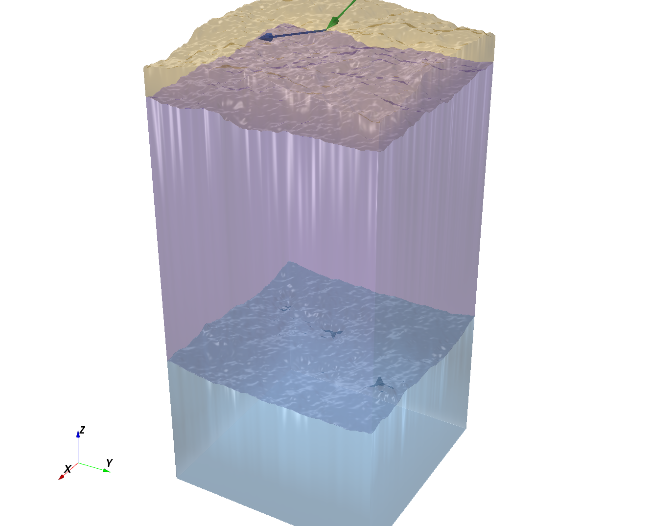
    ba.showSample3D(get_sample(), sample_size=80*nm, seed=0)
    # polarizer and analyzer efficiencies
    p_eff = 0.986
    a_trans = 0.970
    a_supp = 0.015

    results_pp = simulate(R3(0, +1, 0), R3(0, +1, 0), p_eff, a_trans, a_supp, "$++$")
    results_pm = simulate(R3(0, +1, 0), R3(0, -1, 0), p_eff, a_trans, a_supp, "$+-$")
    results_mp = simulate(R3(0, -1, 0), R3(0, +1, 0), p_eff, a_trans, a_supp, "$-+$")
    results_mm = simulate(R3(0, -1, 0), R3(0, -1, 0), p_eff, a_trans, a_supp, "$--$")

    results = [results_pp, results_pm, results_mp, results_mm]
    ba.plot_multicurve(results)
    ba.plt.show()
|
 BornAgain
≻ git-develop
≻ Documentation ≻ Examples ≻ Specular ≻ Magnetic and polarized ≻ Magnetic layer imperfect
BornAgain
≻ git-develop
≻ Documentation ≻ Examples ≻ Specular ≻ Magnetic and polarized ≻ Magnetic layer imperfect