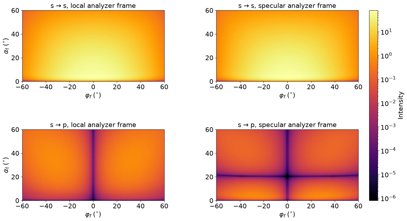
1
 2
 3
 4
 5
 6
 7
 8
 9
10
11
12
13
14
15
16
17
18
19
20
21
22
23
24
25
26
27
28
29
30
31
32
33
34
35
36
37
38
39
40
41
42
43
44
45
46
47
48
49
50
51
52
53
54
55
56
57
58
59
60
61
62
63
64
65
66
67
68
69
70
71
72
73
74
75
76
77
78
79
80
81
82
83
84
85
86
87
88
89
90
|
#!/usr/bin/env python3
# /// script
# requires-python = ">=3.10"
# dependencies = ["bornagain>=25,<26"]
# ///
"""
GISAXS of extreme ultraviolet light (13.5 nm) from molybdenum nanospheres on
silicon, for an s-polarized beam and analyzers for s or p, in the local and in
the specular frame.

A local analyzer faces each outgoing ray and selects its s or p, defined by
that ray and the surface normal. A specular analyzer stays fixed, facing the
nominal specular ray. For each outgoing ray, it selects the normalized
projection of its state perpendicular to that ray. In free space, in Born
approximation, the field radiated by a particle is the projection of the
incident field onto the plane normal to the outgoing ray, so that the
specular s analyzer passes all of it, while the local one misses its p
component outside the plane of incidence. Waves reflected and refracted by
the substrate modify this relation; still, the specular s analyzer receives
nearly everything here. Outside the plane of incidence, the projections of s
and p are not orthogonal, so that the specular s → s and s → p maps do not
add up to the intensity without analyzer. In the plane of incidence, both
frames agree for s and p analyzers.
"""
import bornagain as ba
ba.require_versions("bornagain>=25,<26")
from bornagain import deg, nm, nm2


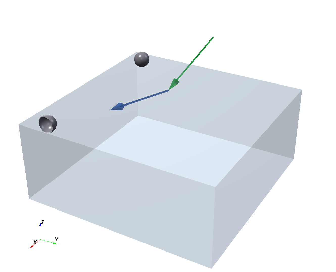
def get_sample():
    """
    Molybdenum spheres on a silicon substrate, with optical constants at
    13.5 nm from the Henke tables.
    """
    molybdenum_color = (0.55, 0.55, 0.6)
    molybdenum = ba.RefractiveMaterial("Mo", molybdenum_color, 0.0762, 0.00644)
    silicon_color = (0.65, 0.75, 0.85)
    silicon = ba.RefractiveMaterial("Si", silicon_color, 0.00100, 0.00183)

    sphere = ba.Particle(molybdenum, ba.Sphere(5*nm))
    layer = ba.Layer(ba.Vacuum())
    layer.deposit2D(ba.Dilute2D(1e-4/nm2, sphere))

    sample = ba.Sample()
    sample.addLayer(layer)
    sample.addLayer(ba.Layer(silicon))
    return sample


def get_simulation(sample, analyzer, frame):
    """
    A GISAXS simulation for an s beam, with a linear analyzer at the given angle
    from s toward p, in the given frame.
    """
    n = 200
    beam = ba.Beam(1e9, 13.5*nm, 20*deg)
    beam.setXrayPolarization(angle=0, axis_ratio=0, degree=1)
    detector = ba.SphericalDetector(n, -60*deg, 60*deg, n, 0, 60*deg)
    detector.setXrayAnalyzer(angle=analyzer, axis_ratio=0, frame=frame)
    simulation = ba.ScatteringSimulation(beam, sample, detector)
    return simulation


def simulate(sample, analyzer, frame, title):
    """
    Runs one combination of analyzer and frame.
    """
    result = get_simulation(sample, analyzer, frame).simulate()
    result.setTitle(title)
    return result


if __name__ == '__main__':
    sample = get_sample()
    # Angles of s and p polarization
    s_wave = 0
    p_wave = 90*deg
    settings = [
        ("s → s, local analyzer frame", s_wave, "local"),
        ("s → s, specular analyzer frame", s_wave, "specular"),
        ("s → p, local analyzer frame", p_wave, "local"),
        ("s → p, specular analyzer frame", p_wave, "specular"),
    ]
    results = [
        simulate(sample, analyzer, frame, title)
        for title, analyzer, frame in settings
    ]
    ba.showSample3D(sample, sample_size=120*nm, seed=0)
    ba.plot2d_to_grid(results, 2, unit_aspect=1)
    ba.plt.show()
|
 BornAgain
≻ git-develop
≻ Documentation ≻ Examples ≻ GISAS ≻ Simulation setup and instrument ≻ X-ray analyzer frame