The interference function of a radial paracrystal is used to model cumulative disorder of interparticle distances. It is called radial to stress the fact that it only takes into account the radial component of the scattering vector.
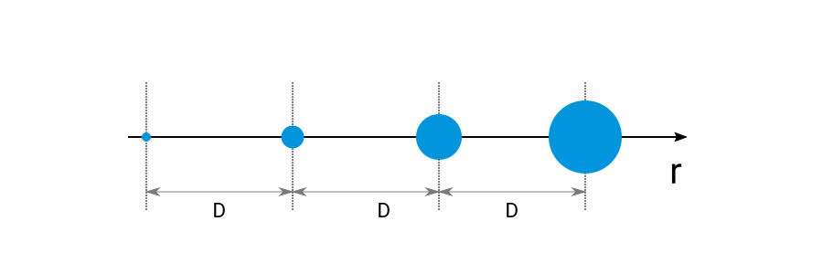
Each circle on the plot above represents the area where the probability to find a particle, given a particle at the origin, is above some arbitrary threshold. The growing size of the areas emphasizes the fact the our knowledge about next neighbor’s location decreases with the distance to the origin.
The BornAgain user manual (Chapter 3.5, Paracrystal) details the theoretical model and gives some links to the literature.
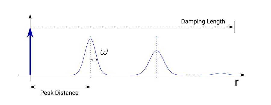
The radial paracrystal is parameterized by the position distribution of the nearest neighbor centered at the peak distance. On the plot below the half-width of this distribution is marked as $\omega$ and the center is marked with “Peak Distance”. The probability distributions of finding other particles to the right are deduced from accumulating position uncertanties of previous particles in the chain.
To create the interference function of a radial paracrystal the following constructor has to be used.
RadialParacrystal(peak_distance, damping_length=0)
"""
peak_distance   Average distance to the next neighbor in nanometers
damping_length  The damping (coherence) length of the paracrystal in nanometers.
"""
The parameter damping_length is used to introduce finite size
effects by applying a multiplicative coefficient equal to
$exp \left(-\frac{peak\_distance}{damping\_length}\right)$
to the Fourier transform of the probability density of a nearest neighbor.
damping_length is equal to 0 by default and, in this case, no correction is applied.
On the plot above the damping length is provisionally depicted as
an area contributing to the scattering.
To account for next neighbor position uncertainty a probability
distribution should be assigned to the interference function.
This is done using the setProbabilityDistribution(pdf) method
of the radial paracrystal interference function.
iff = ba.RadialParacrystal(10.0*nm, 1000.0*nm)
iff.setProbabilityDistribution(ba.Profile1DCauchy(30.0*nm))
The following distributions are available
# Cauchy-Lorentzian distribution
ba.Profile1DCauchy(omega)

# Gaussian distribution
ba.Profile1DGauss(omega)

# gate distribution
ba.Profile1DGate(omega)

# triangle distribution
ba.Profile1DTriangle(omega)

# cosine distribution
ba.Profile1DCosine(omega)

# pseudo-Voigt distribution: eta*Gauss + (1-eta)*Cauchy
Profile1DVoigt(omega, eta)
The parameter omega is used to set the half-width of the distribution in nanometers.
In the case of the pseudo-Voigt distribution an additional dimensionless parameter
eta is used to balance between the Gaussian and Cauchy profiles.
The interference function of a radial paracrystal provides a way to calculate
the scattering from a finite portion of the paracrystal using the
setDomainSize(nm) method. The resulting behaviour is similar to the case when
damping_length is used (the difference in computation is explained in the user manual).
In the code snippet below, the paracrystal is created without specifying the
damping_length, and then the setDomainSize method is used to introduce
the alternative mechanism for finite size corrections.
iff = RadialParacrystal(10.0*nm)
iff.setProbabilityDistribution(Profile1DCauchy(30.0*nm))
iff.setDomainSize(10000*nm)
During the simulation setup the particle density has to be explicitly specified
by the user for correct normalization of overall intensity.
This is done by using ParticleLayout.setParticleDensity(density) method.
The density parameter is given here in “number of particles per square nanometer”.
The radial paracrystal model is used to demonstrate the differences in size-distribution models