  1
  2
  3
  4
  5
  6
  7
  8
  9
 10
 11
 12
 13
 14
 15
 16
 17
 18
 19
 20
 21
 22
 23
 24
 25
 26
 27
 28
 29
 30
 31
 32
 33
 34
 35
 36
 37
 38
 39
 40
 41
 42
 43
 44
 45
 46
 47
 48
 49
 50
 51
 52
 53
 54
 55
 56
 57
 58
 59
 60
 61
 62
 63
 64
 65
 66
 67
 68
 69
 70
 71
 72
 73
 74
 75
 76
 77
 78
 79
 80
 81
 82
 83
 84
 85
 86
 87
 88
 89
 90
 91
 92
 93
 94
 95
 96
 97
 98
 99
100
101
102
103
104
105
106
107
108
109
110
111
112
113
114
115
116
117
118
119
120
121
122
123
124
125
126
127
128
129
130
131
132
133
134
135
136
137
138
139
140
141
142
143
144
145
146
147
148
149
150
151
152
153
154
155
156
157
158
159
160
161
162
163
164
165
166
167
168
169
170
171
172
173
174
175
176
177
178
179
180
181
182
183
184
185
186
187
188
189
190
191
192
193
194
195
196
197
198
199
200
201
202
203
204
205
206
207
208
209
210
211
212
213
214
215
216
217
218
219
220
221
222
223
224
225
226
227
228
229
230
231
232
233
234
235
236
237
238
239
240
241
242
243
244
245
246
247
248
249
250
251
252
253
254
255
256
257
258
259
260
261
262
263
264
265
266
267
268
269
270
271
272
273
274
275
276
277
278
279
280
281
282
283
284
285
286
287
288
289
290
291
292
293
294
295
296
297
298
299
300
301
302
303
304
305
306
307
308
309
310
311
312
313
314
315
316
317
318
319
320
321
322
323
324
325
326
327
328
329
330
331
332
333
334
335
336
337
338
339
340
341
342
343
344
345
346
347
348
349
350
351
352
353
354
355
356
357
358
359
360
361
362
363
364
365
366
367
368
369
370
371
372
373
374
375
376
377
378
|
#!/usr/bin/env python3
"""
This fitting and simulation example demonstrates how to replicate
the fitting example "Magnetically Dead Layers in Spinel Films"
given at the Nist website:
https://www.nist.gov/ncnr/magnetically-dead-layers-spinel-films
For simplicity, here we only reproduce the first part of that
demonstration without the magnetically dead layer.
"""
# import boranagain
import bornagain as ba
from bornagain import deg, angstrom, nm
import numpy
import matplotlib.pyplot as plt
# import more libs needed for data processing
from re import match, DOTALL
from sys import argv
from io import BytesIO
from urllib.request import urlopen
from zipfile import ZipFile
from os.path import isfile
# q-range on which the simulation and fitting are to be performed
qmin = 0.05997
qmax = 1.96
# number of points on which the computed result is plotted
scan_size = 1500
# The SLD of the substrate is kept constant
sldMao = (5.377e-06, 0)
# constant to convert between magnetization and magnetic SLD
RhoMconst = 2.910429812376859e-12
####################################################################
# Create Sample and Simulation #
####################################################################
def get_sample(params):
"""
construct the sample with the given parameters
"""
magnetizationMagnitude = params["rhoM_Mafo"]*1e-6/RhoMconst
angle = 0
magnetizationVector = ba.kvector_t(
magnetizationMagnitude*numpy.sin(angle*deg),
magnetizationMagnitude*numpy.cos(angle*deg), 0)
mat_vacuum = ba.MaterialBySLD("Vacuum", 0, 0)
mat_layer = ba.MaterialBySLD("(Mg,Al,Fe)3O4", params["rho_Mafo"]*1e-6,
0, magnetizationVector)
mat_substrate = ba.MaterialBySLD("MgAl2O4", *sldMao)
ambient_layer = ba.Layer(mat_vacuum)
layer = ba.Layer(mat_layer, params["t_Mafo"]*angstrom)
substrate_layer = ba.Layer(mat_substrate)
r_Mafo = ba.LayerRoughness()
r_Mafo.setSigma(params["r_Mafo"]*angstrom)
r_substrate = ba.LayerRoughness()
r_substrate.setSigma(params["r_Mao"]*angstrom)
multi_layer = ba.MultiLayer()
multi_layer.addLayer(ambient_layer)
multi_layer.addLayerWithTopRoughness(layer, r_Mafo)
multi_layer.addLayerWithTopRoughness(substrate_layer, r_substrate)
return multi_layer
def get_simulation(q_axis, parameters, polarization, analyzer):
"""
Returns a simulation object.
Polarization, analyzer and resolution are set
from given parameters
"""
simulation = ba.SpecularSimulation()
q_axis = q_axis + parameters["q_offset"]
scan = ba.QSpecScan(q_axis)
dq = parameters["q_res"]*q_axis
n_sig = 4.0
n_samples = 25
distr = ba.RangedDistributionGaussian(n_samples, n_sig)
scan.setAbsoluteQResolution(distr, parameters["q_res"])
simulation.beam().setPolarization(polarization)
simulation.setAnalyzerProperties(analyzer, 1, 0.5)
simulation.setScan(scan)
return simulation
def run_simulation(q_axis, fitParams, *, polarization, analyzer):
"""
Run a simulation on the given q-axis, where the sample is constructed
with the given parameters.
Vectors for polarization and analyzer need to be provided
"""
parameters = dict(fitParams, **fixedParams)
sample = get_sample(parameters)
simulation = get_simulation(q_axis, parameters, polarization, analyzer)
simulation.setSample(sample)
simulation.runSimulation()
return simulation
def qr(result):
"""
Returns two arrays that hold the q-values as well as the
reflectivity from a given simulation result
"""
q = numpy.array(result.result().axis(ba.Axes.QSPACE))
r = numpy.array(result.result().array(ba.Axes.QSPACE))
return q, r
####################################################################
# Plot Handling #
####################################################################
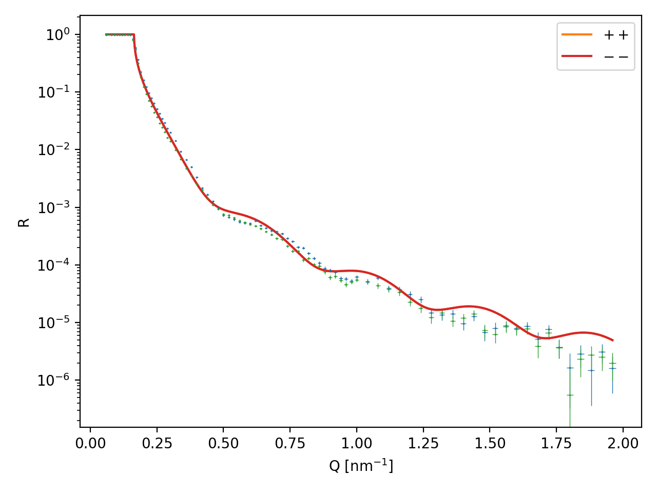
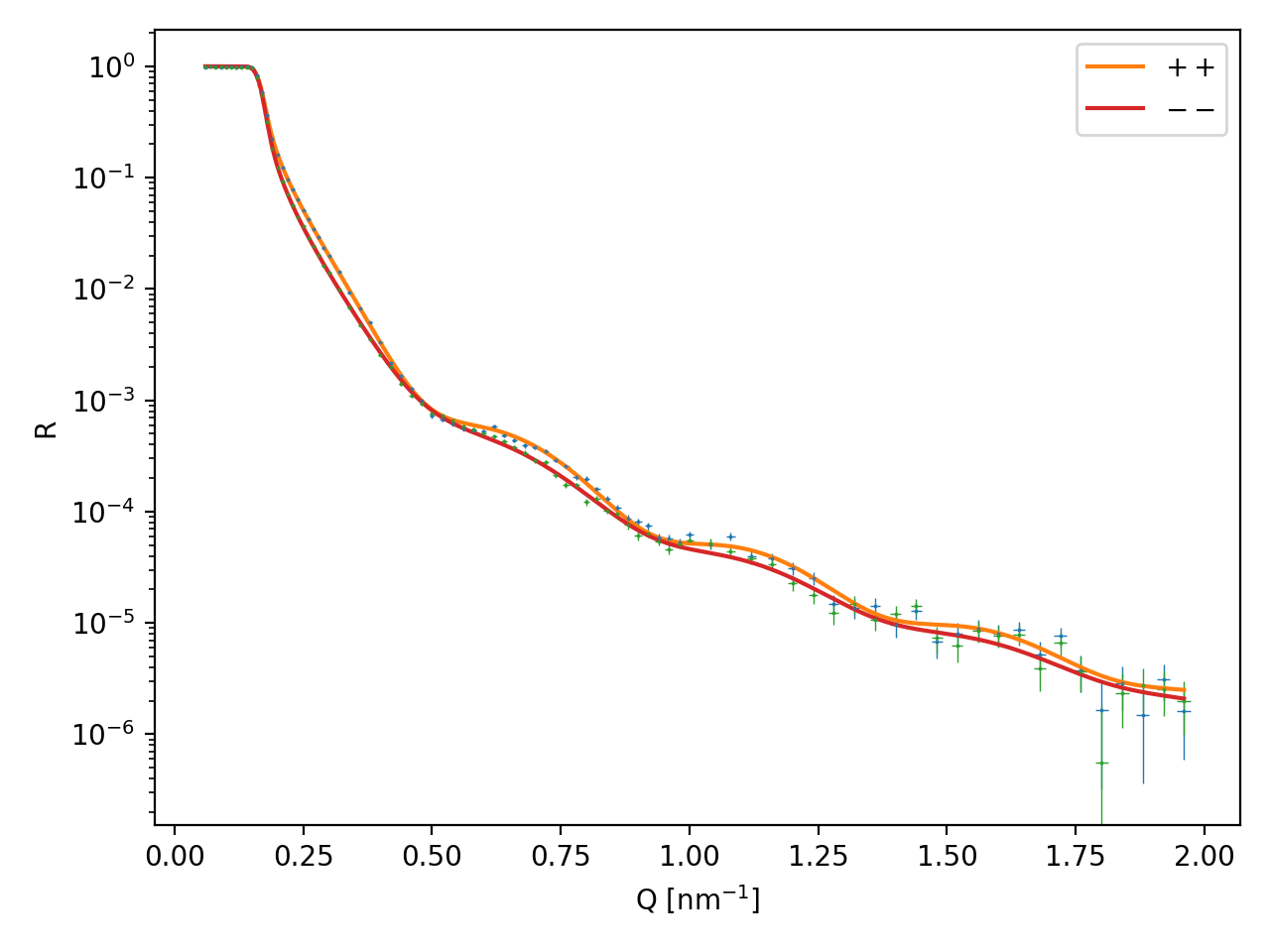
def plot(qs, rs, exps, labels, filename):
"""
Plot the simulated result together with the experimental data
"""
fig = plt.figure()
ax = fig.add_subplot(111)
for q, r, exp, l in zip(qs, rs, exps, labels):
ax.errorbar(exp[0],
exp[1],
xerr=exp[3],
yerr=exp[2],
fmt='.',
markersize=0.75,
linewidth=0.5)
ax.plot(q, r, label=l)
ax.set_yscale('log')
plt.legend()
plt.xlabel("Q [nm${}^{-1}$]")
plt.ylabel("R")
plt.tight_layout()
plt.savefig(filename)
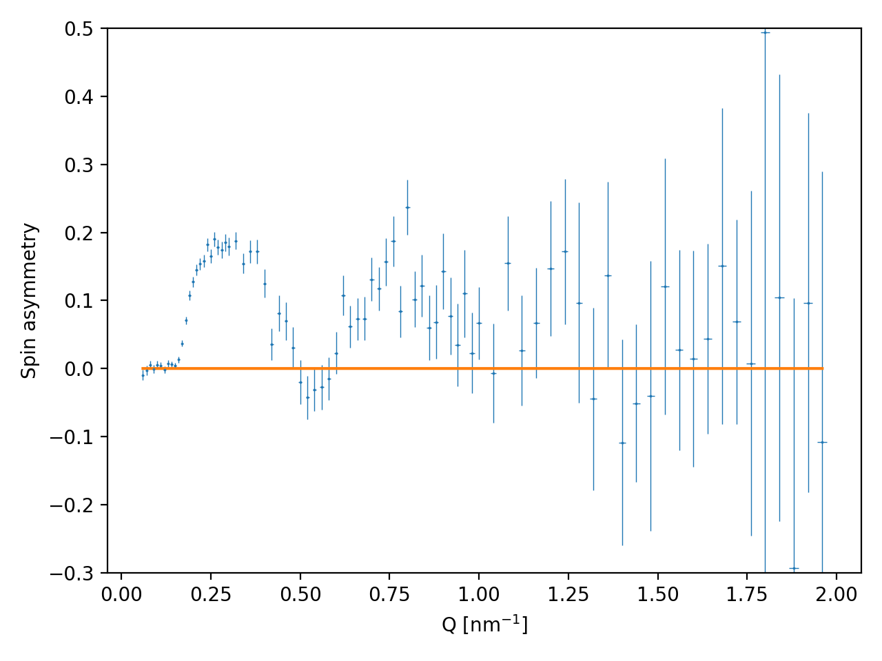
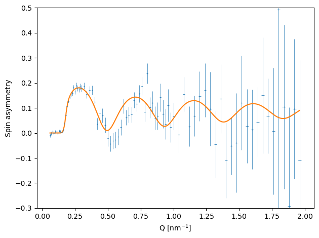
def plotSpinAsymmetry(data_pp, data_mm, q, r_pp, r_mm, filename):
"""
Plot the simulated spin asymmetry as well its
experimental counterpart with errorbars
"""
# compute the errorbars of the spin asymmetry
delta = numpy.sqrt(4 * (data_pp[1]**2 * data_mm[2]**2 + \
data_mm[1]**2 * data_pp[2]**2 ) /
( data_pp[1] + data_mm[1] )**4 )
fig = plt.figure()
ax = fig.add_subplot(111)
ax.errorbar(data_pp[0],
(data_pp[1] - data_mm[1])/(data_pp[1] + data_mm[1]),
xerr=data_pp[3],
yerr=delta,
fmt='.',
markersize=0.75,
linewidth=0.5)
ax.plot(q, (r_pp - r_mm)/(r_pp + r_mm))
plt.gca().set_ylim((-0.3, 0.5))
plt.xlabel("Q [nm${}^{-1}$]")
plt.ylabel("Spin asymmetry")
plt.tight_layout()
plt.savefig(filename)
####################################################################
# Data Handling #
####################################################################
def normalizeData(data):
"""
Removes duplicate q values from the input data,
normalizes it such that the maximum of the reflectivity is
unity and rescales the q-axis to inverse nm
"""
r0 = numpy.where(data[0] - numpy.roll(data[0], 1) == 0)
data = numpy.delete(data, r0, 1)
data[0] = data[0]/angstrom
data[3] = data[3]/angstrom
norm = numpy.max(data[1])
data[1] = data[1]/norm
data[2] = data[2]/norm
so = numpy.argsort(data[0])
data = data[:, so]
return data
def filterData(data, qmin, qmax):
minIndex = numpy.argmin(numpy.abs(data[0] - qmin))
maxIndex = numpy.argmin(numpy.abs(data[0] - qmax))
return data[:, minIndex:maxIndex + 1]
def get_Experimental_data(qmin, qmax):
input_Data = downloadAndExtractData()
data_pp = normalizeData(input_Data[0])
data_mm = normalizeData(input_Data[1])
return (filterData(data_pp, qmin,
qmax), filterData(data_mm, qmin, qmax))
def downloadAndExtractData():
url = "https://www.nist.gov/document/spinelfilmzip"
if not isfile("spinelfilm.zip"):
downloadfile = urlopen(url)
with open("spinelfilm.zip", 'wb') as outfile:
outfile.write(downloadfile.read())
zipfile = ZipFile("spinelfilm.zip")
rawdata = zipfile.open("MAFO_Saturated.refl").read().decode("utf-8")
table_pp = match(
r'.*# "polarization": "\+\+"\n#.*?\n# "units".*?\n(.*?)#.*',
rawdata, DOTALL).group(1)
table_mm = match(
r'.*# "polarization": "\-\-"\n#.*?\n# "units".*?\n(.*?)#.*',
rawdata, DOTALL).group(1)
data_pp = numpy.genfromtxt(BytesIO(table_pp.encode()), unpack=True)
data_mm = numpy.genfromtxt(BytesIO(table_mm.encode()), unpack=True)
return (data_pp, data_mm)
####################################################################
# Fit Function #
####################################################################
def run_fit_ba(q_axis, r_data, r_uncertainty, simulationFactory,
startParams):
fit_objective = ba.FitObjective()
fit_objective.setObjectiveMetric("chi2")
fit_objective.addSimulationAndData(
lambda params: simulationFactory[0](q_axis[0], params), r_data[0],
r_uncertainty[0], 1)
fit_objective.addSimulationAndData(
lambda params: simulationFactory[1](q_axis[1], params), r_data[1],
r_uncertainty[1], 1)
fit_objective.initPrint(10)
params = ba.Parameters()
for name, p in startParams.items():
params.add(name, p[0], min=p[1], max=p[2])
minimizer = ba.Minimizer()
result = minimizer.minimize(fit_objective.evaluate, params)
fit_objective.finalize(result)
return {r.name(): r.value for r in result.parameters()}
####################################################################
# Main Function #
####################################################################
if __name__ == '__main__':
if len(argv) > 1 and argv[1] == "fit":
fixedParams = {
# parameters can be moved here to keep them fixed
}
fixedParams = {d: v[0] for d, v in fixedParams.items()}
startParams = {
# own starting values
"q_res": (0, 0, 0.1),
"q_offset": (0, -0.002, 0.002),
"rho_Mafo": (6.3649, 2, 7),
"rhoM_Mafo": (0, 0, 2),
"t_Mafo": (150, 60, 180),
"r_Mao": (1, 0, 12),
"r_Mafo": (1, 0, 12),
}
fit = True
else:
startParams = {}
fixedParams = {
# parameters from our own fit run
'q_res': 0.010542945012551425,
'q_offset': 7.971243487467318e-05,
'rho_Mafo': 6.370140108715461,
'rhoM_Mafo': 0.27399566816062926,
't_Mafo': 137.46913056084736,
'r_Mao': 8.60487712674644,
'r_Mafo': 3.7844265311293483
}
fit = False
paramsInitial = {d: v[0] for d, v in startParams.items()}
def run_Simulation_pp(qzs, params):
return run_simulation(qzs,
params,
polarization=ba.kvector_t(0, 1, 0),
analyzer=ba.kvector_t(0, 1, 0))
def run_Simulation_mm(qzs, params):
return run_simulation(qzs,
params,
polarization=ba.kvector_t(0, -1, 0),
analyzer=ba.kvector_t(0, -1, 0))
qzs = numpy.linspace(qmin, qmax, scan_size)
q_pp, r_pp = qr(run_Simulation_pp(qzs, paramsInitial))
q_mm, r_mm = qr(run_Simulation_mm(qzs, paramsInitial))
data_pp, data_mm = get_Experimental_data(qmin, qmax)
plot([q_pp, q_mm], [r_pp, r_mm], [data_pp, data_mm], ["$++$", "$--$"],
f'MAFO_Saturated_initial.pdf')
plotSpinAsymmetry(data_pp, data_mm, qzs, r_pp, r_mm,
"MAFO_Saturated_spin_asymmetry_initial.pdf")
if fit:
fitResult = run_fit_ba([data_pp[0], data_mm[0]],
[data_pp[1], data_mm[1]],
[data_pp[2], data_mm[2]],
[run_Simulation_pp, run_Simulation_mm],
startParams)
print("Fit Result:")
print(fitResult)
q_pp, r_pp = qr(run_Simulation_pp(qzs, fitResult))
q_mm, r_mm = qr(run_Simulation_mm(qzs, fitResult))
plot([q_pp, q_mm], [r_pp, r_mm], [data_pp, data_mm],
["$++$", "$--$"], f'MAFO_Saturated_fit.pdf')
plotSpinAsymmetry(data_pp, data_mm, qzs, r_pp, r_mm,
"MAFO_Saturated_spin_asymmetry_fit.pdf")
|