3D nanoparticle arrangements obtained using different techniques are complex, but quite frequent kinds of samples being studied with GISAS. Depending on the properties of the particular sample you may choose one of 2 ways to represent a 3D particle arrangement in a BornAgain simulation:
Below you will find a detailed description of each option.
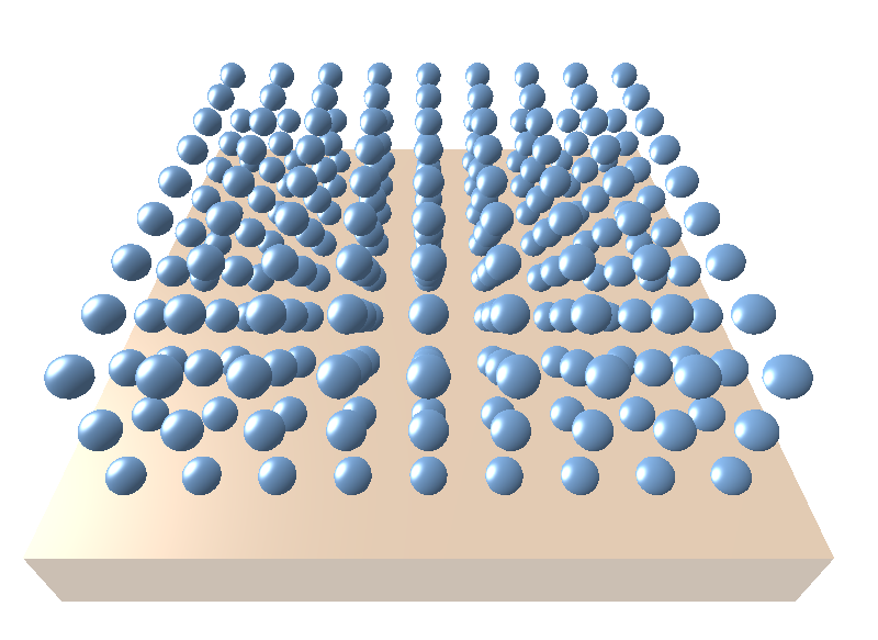
Let’s take a case of spherical particles arranged in a cubic lattice with the following parameters:
particle_radius = 2.5*nm
lattice_length = 10.0*nm
height = 50.0*nm
One can easily create such a structure either in GUI or in Python using the following steps:
Create a particle composition
# Defining Form Factors
ff_sphere = ba.FormFactorFullSphere(particle_radius)

# Defining composition of particles at specific positions
particle_composition = ba.ParticleComposition()

# compute number of particles in the vertical direction
n = int((height - 2.0*particle_radius) // lattice_length)

# add particles to the particle composition
for i in range(n+1):
    particle = ba.Particle(m_particle, ff_sphere)
    particle_position = kvector_t(0.0*nm, 0.0*nm, i*lattice_length)
    particle.setPosition(particle_position)
    particle_composition.addParticle(particle)
If you work in GUI, you will need to add each particle manually. See the Particle composition tutorial for more details.
Arrange created compositions in a lattice.
For this example we will use a 2D square lattice.
# Defining Interference Function
interference = ba.InterferenceFunction2DLattice(lattice_length, lattice_length, 90.0*deg, 0.0*deg)
interference_pdf = ba.FTDecayFunction2DCauchy(500.0*nm, 500.0*nm, 0.0*deg)
interference.setDecayFunction(interference_pdf)

# Defining Particle Layout and adding Particles
layout = ba.ParticleLayout()
layout.addParticle(particle_composition, 1.0)
layout.setInterferenceFunction(interference)
See the Interference functions tutorial for more details on interference functions available in BornAgain.
Often, the particle arrangement over the sample is not uniform, but consists of domains rotated with respect to each other. This will influence the number and positions of interference peaks in the observed GISAS pattern.
If you assume a uniform rotational distribution of the domains, you can consider it in the simulation using the following Python code:
interference.setIntegrationOverXi(True)
or by activating a corresponding checkbox in the GUI. Pay attention, this setting will slow down the simulation dramatically.
If you suggest that domains in your sample have a preferred orientation, you can create the rotational distribution manually. For this purpose you will need to modify the Python code as follows. First, we introduce the lattice rotations dictionary
# lattice rotations dictionary, consists of pairs "xi: weight"
# sum of the weights must be less or equal to 1
rotations = {0.0: 0.7, 45.0: 0.3}
In this example we consider two lattice rotations: $\xi=0^{\circ}$ with weight 0.7 and $\xi=45^{\circ}$ with weight 0.3. Pay attention, BornAgain requires that the sum of layout weights to be less than or equal to 1. To add these layouts to the multilayer, we modify the Python code as follows:
for xi in rotations.keys():
    # Defining Interference Function
    interference = ba.InterferenceFunction2DLattice(lattice_length, lattice_length, 90.0*deg, xi*deg)
    interference_pdf = ba.FTDecayFunction2DCauchy(500.0*nm, 500.0*nm, 0.0*deg)
    interference.setDecayFunction(interference_pdf)

    # Defining Particle Layout and adding Particles
    layout = ba.ParticleLayout()
    layout.addParticle(particle_composition, 1.0)
    layout.setInterferenceFunction(interference)
    layout.setWeight(rotations[xi])

    # Adding layouts to layers
    l_air.addLayout(layout)
In the GUI you should create and add all the layouts manually. This approach makes sense if you have just a few rotations.
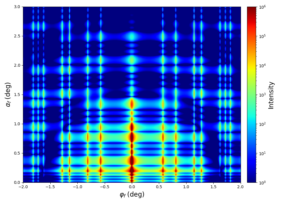
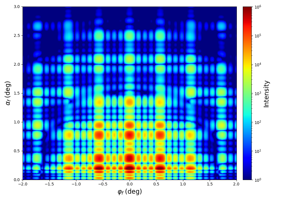
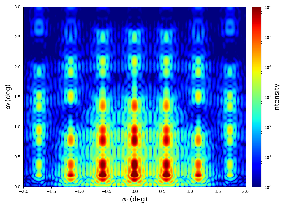
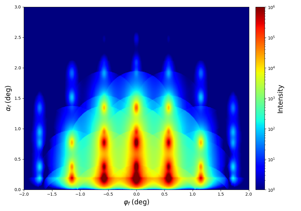
Uniform rotational distribution
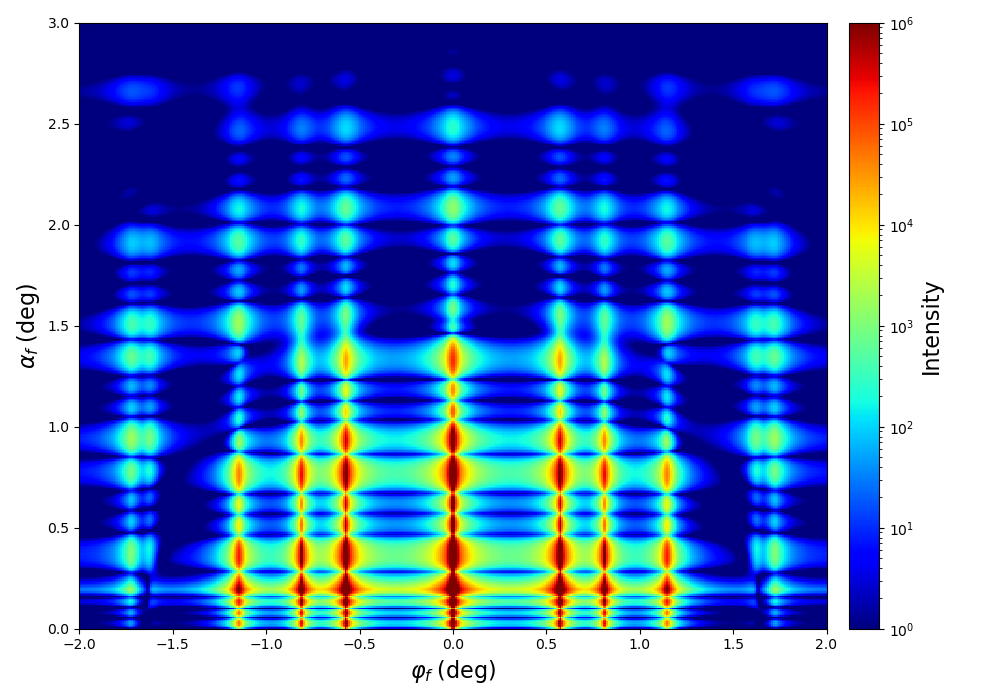
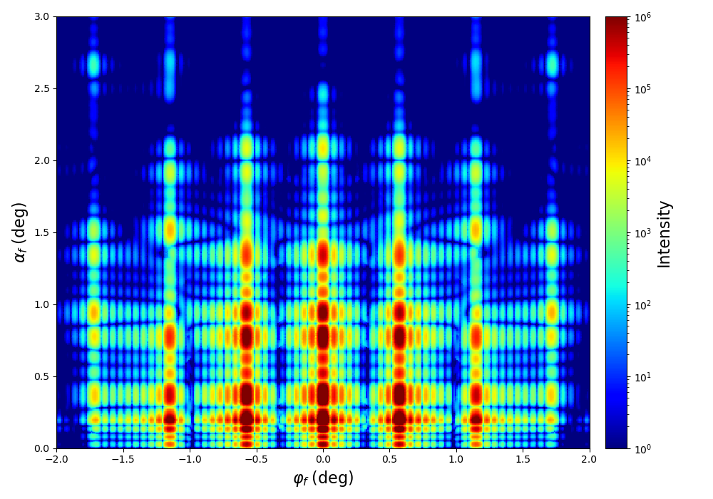
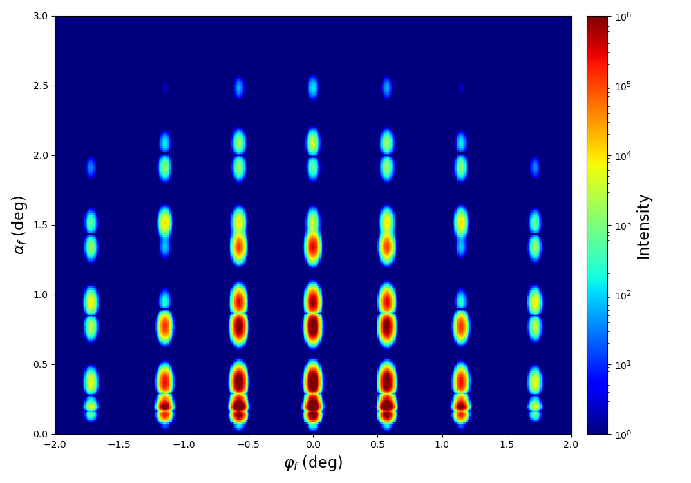
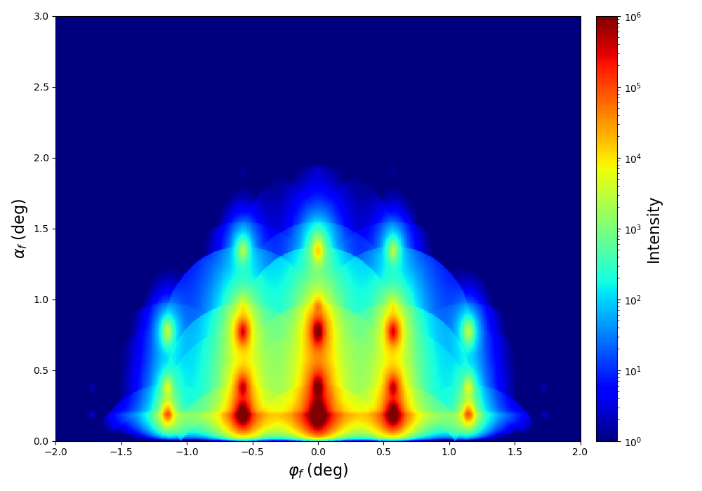
Two lattice rotation angles
Figures above show the influence of both considered rotational distributions on the GISAS pattern.
Alternatively, you can consider to use distributions available in BornAgain. See the Particle distribution tutorial for more information. In this case you should apply the chosen distribution to the parameter Interference2DLattice/BasicLattice/Xi. See the corresponding tutorial example for details.
If your particle composition is not symmetrical, you may need to rotate your particles as well. See the Particle rotation tutorial for details.
Complete Python scripts for this part of tutorial
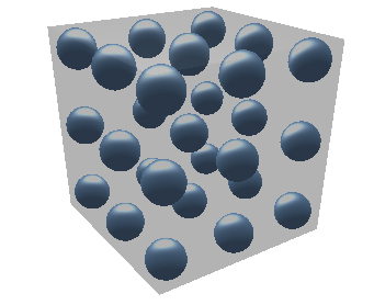
Another and more flexible way to represent a 3D particle arrangement is as a mesocrystal. It can be easily created in both, GUI and Python. The complete Python script to create a mesocrystal you can find in the Mesocrystal tutorial.
In the present tutorial, we consider a mesocrystal with the following parameters
# parameters of 3D particle arrangement
particle_radius = 2.50*nm
lattice_length = 10.0*nm
# mesocrystal size
meso_height = 50.0nm
meso_width = 500.0nm
meso_length = 500.0*nm
Mesocrystal can be created in the following steps.
Create particles that form the base of the mesocrystal
# Spherical particles, form the base of the mesocrystal
ff_sphere = ba.FormFactorFullSphere(particle_radius)
sphere = ba.Particle(m_particle, ff_sphere)
Create lattice
# mesocrystal lattice (cubic lattice for this example)
lattice_a = ba.kvector_t(lattice_length, 0.0, 0.0)
lattice_b = ba.kvector_t(0.0, lattice_length, 0.0)
lattice_c = ba.kvector_t(0.0, 0.0, lattice_length)
lattice = ba.Lattice(lattice_a, lattice_b, lattice_c)
Create a mesocrystal
# crystal structure
crystal = ba.Crystal(sphere, lattice)
# mesocrystal
meso_ff = ba.FormFactorBox(meso_length, meso_width, meso_height)
meso = ba.MesoCrystal(crystal, meso_ff)
layout = ba.ParticleLayout()
layout.addParticle(meso)
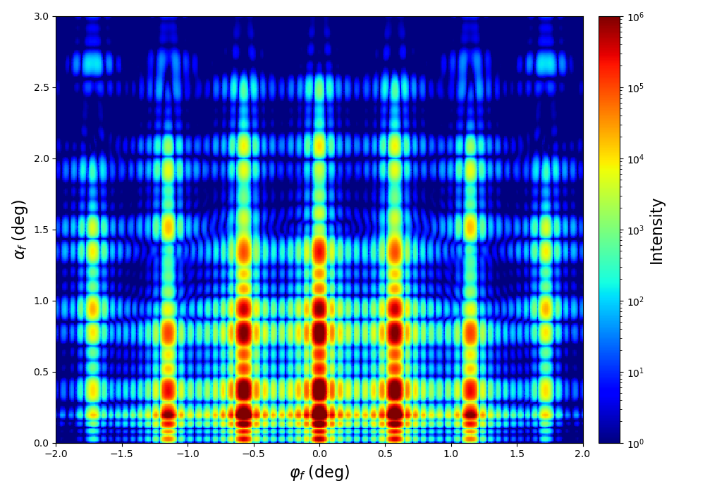
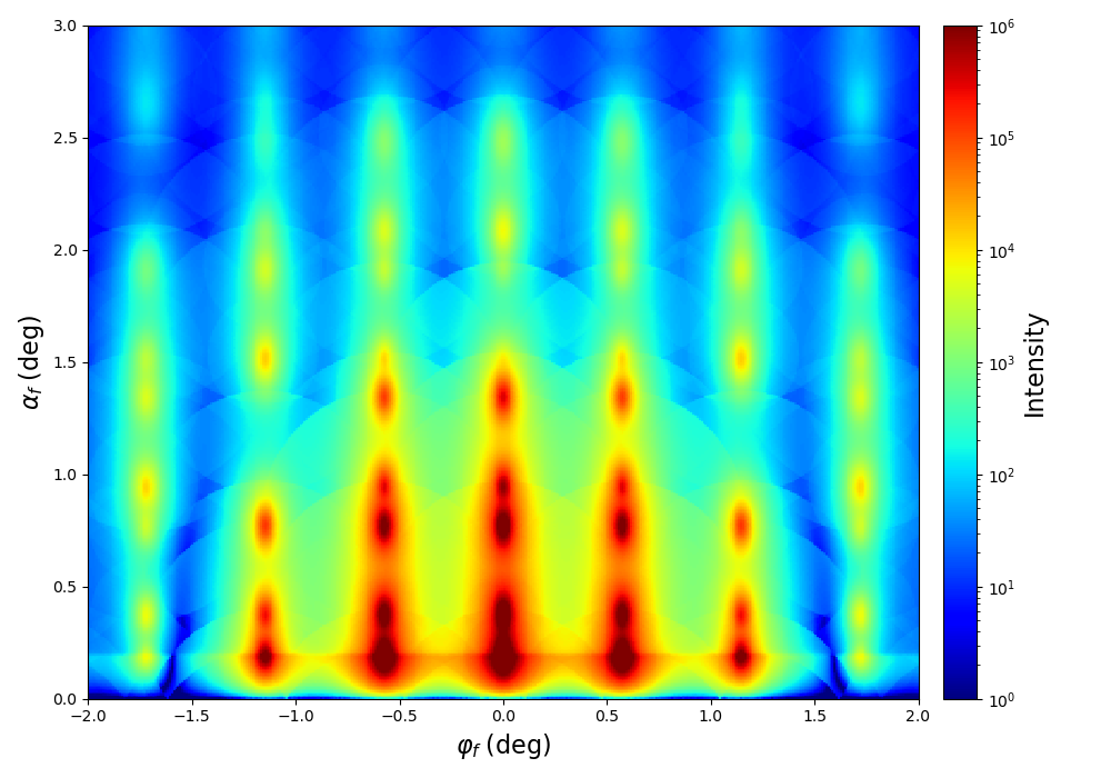
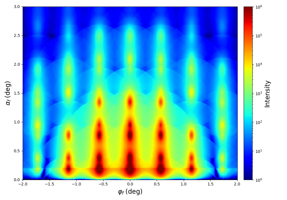
The size of the mesocrystal influences the GISAS pattern dramatically. This is especially well seen for small mesocrystals. Unless you know size of your mesocrystals from other techniques, we recommend to vary it to find the one that matches the experimental data the best.
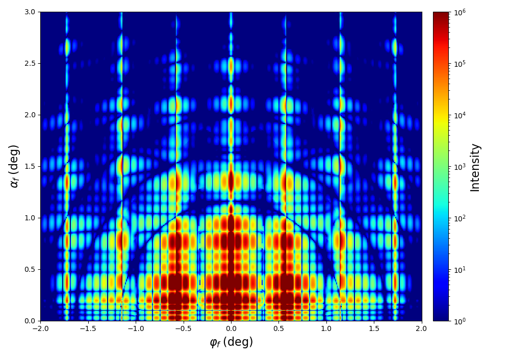
Mesocrystal of $W=L=50$ nm
Mesocrystal of $W=L=100$ nm
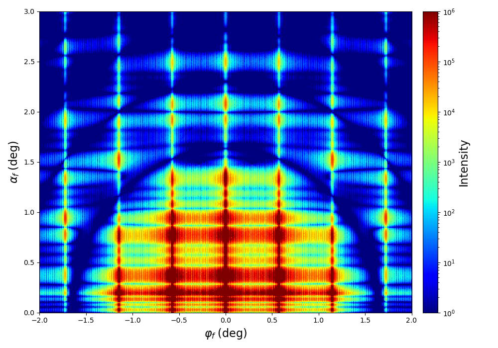
Mesocrystal of $W=L=250$ nm

Mesocrystal of $W=L=500$ nm
In the figures above, you can see the GISAS pattern for a Box-shaped mesocrystal of different sizes in lateral direction. For simplicity, we take width $W$ and length $L$ of the mesocrystal equal. As you can see, small mesocrystals cause a lot of peaks coming from the mesocrystal shape. These peaks “vanish” for large mesocrystals, because the intensity starts to oscillate so fast, that we are not able anymore to observe them. You can also see, that the shape of the “structure” peaks is also affected.
The shape of the mesocrystal is also a very important parameter that influences the GISAS pattern. To vary the shape you can choose any of the particle form factors available in BornAgain. See the example on available particle form factors
Cylinder
Truncated Sphere
Gauss
Lorentz
The figures above show the GISAS patterns for different shapes of mesocrystals. The width of all mesocrystals is $100$ nm. Form factors FormFactorGauss and FormFactorLorentz are presently not available in GUI. However, they can be used from Python:
meso_ff = ba.FormFactorGauss(meso_width, meso_height)
or
meso_ff = ba.FormFactorLorentz(meso_width, meso_height)
Position variance describes the displacement of the nanoparticle around the lattice point in 3D. The larger the position variance, the stronger will be the attenuation of the peak intensity along $Q_z$. This can be seen in the figures below.
Position variance $0.1$ nm$^2$

Position variance $0.5$ nm$^2$
Position variance $1$ nm$^2$
Position variance $2$ nm$^2$
This setting is presently not available in GUI. It can be used from Python as follows
crystal = ba.Crystal(sphere, lattice)
# crystal.setDWFactor(0.5)  # for BornAgain versions 1.16 and below
crystal.setPositionVariance(0.5)  # for newer BornAgain versions
While representing a 3D nanoparticle arrangement as a mesocrystal, you might come up with a question whether you need an interference function. The answer depends on the size of your mesocrystal, distance between mesocrystals and resolution of the instrument where the measurements are performed.
Let’s take the mesocrystal of width $W=100$ nm and distance between two mesocrystals $D=300$ nm. In this case, to be able to resolve interference peaks you will need an instrument resolution of at least:
$$\Delta Q = \frac{2\pi}{300}\approx\;0.02\; nm^{-1} \approx \; 0.002 \; \unicode{x212B}^{-1}$$
Often you need rather large mesocrystals to represent a 3D nanoparticle arrangement. In this case, the intensity will oscillate over each detector bin with high frequency. Thus, the analytical computation with sampling points in the bin centers will cause artifacts in the simulated GISAS pattern. This is shown in the figures below.
Analytical computation
Monte-Carlo integration
The way to avoid this problem implemented in BornAgain is Monte-Carlo integration over the detector bin. You can switch it on in both, GUI (checkbox in the Simulation view) and in Python
simulation.getOptions().setMonteCarloIntegration(True, n)
where n is a number of points for Monte-Carlo integration. For more details see the Large particle formfactor tutorial.
Download the complete Python script: mesocrystal.py
Besides of Bragg peaks, measured GISAS patterns often contain diffuse scattering. This is a sign of some kind of disorder in the sample. Which kind of disorder it is exactly, depends on the sample production technique. Here we can list some frequent types:
PositionZ). To add loose particles, you will need to create a separate ParticleLayout and add it to the same layer as the mesocrystal with an appropriate weight. For more information about particle distributions, see the particle distribution tutorial.Relative weights of layouts as well as TotalParticleSurfaceDensity in each layout will affect the relative scattering intensities caused by particles of each particle layout. You can set these parameters either in GUI or using the following Python code
layout = ba.ParticleLayout()
layout.addParticle(meso)
layout.setTotalParticleSurfaceDensity(1.0e-04)    # or any other reasonable number between 0 and 1
layout.setWeight(0.5)                             # or any other reasonable number between 0 and 1
Rotation as transformation. In Python, you would need to use the following codemeso = ba.MesoCrystal(crystal, meso_ff)
meso_rotation = ba.RotationZ(45.0*deg)
meso.setRotation(meso_rotation)
This example rotates the mesocrystal around $Z$ axis by 45 degrees. You can also apply a rotational distribution in a way similar to the one described above in the Particle compositions arranged in a lattice section.
Start with a simplest model. If you have simple and well-ordered system, use particle composition. If you observe signs of disorder in experimental data, use mesocrystal. Important is at first to build a simplest possible model that matches peak positions.
If you have heterogeneous nanoparticle arrangements, first check the contrast of all the particles to the medium. If the SLD of some particles does not differ noticeably from the ambient SLD, don’t simulate them. It will allow for a simpler model and will save you computation time. The same approach we recommend for core-shell particles.
If a simulation does not reproduce all the peaks observed in experimental data, try to add a rotational distribution. For the beginning keep it as simple as possible.
If particles in 3D arrangements are densely packed, use averaged materials. It might have a strong influence on the GISAS pattern in the range of small $Q_z$. This can be done either by choosing Average Layer Material in Simulation view in GUI or with the following Python code:
simulation.getOptions().setUseAvgMaterials(True)
See also tutorial examples on Hemispheres in Averaged Layer and Cylinders in Averaged Layer.
Find appropriate sample and instrument parameters to match the simulation with the fake experimental data presented in the figure below
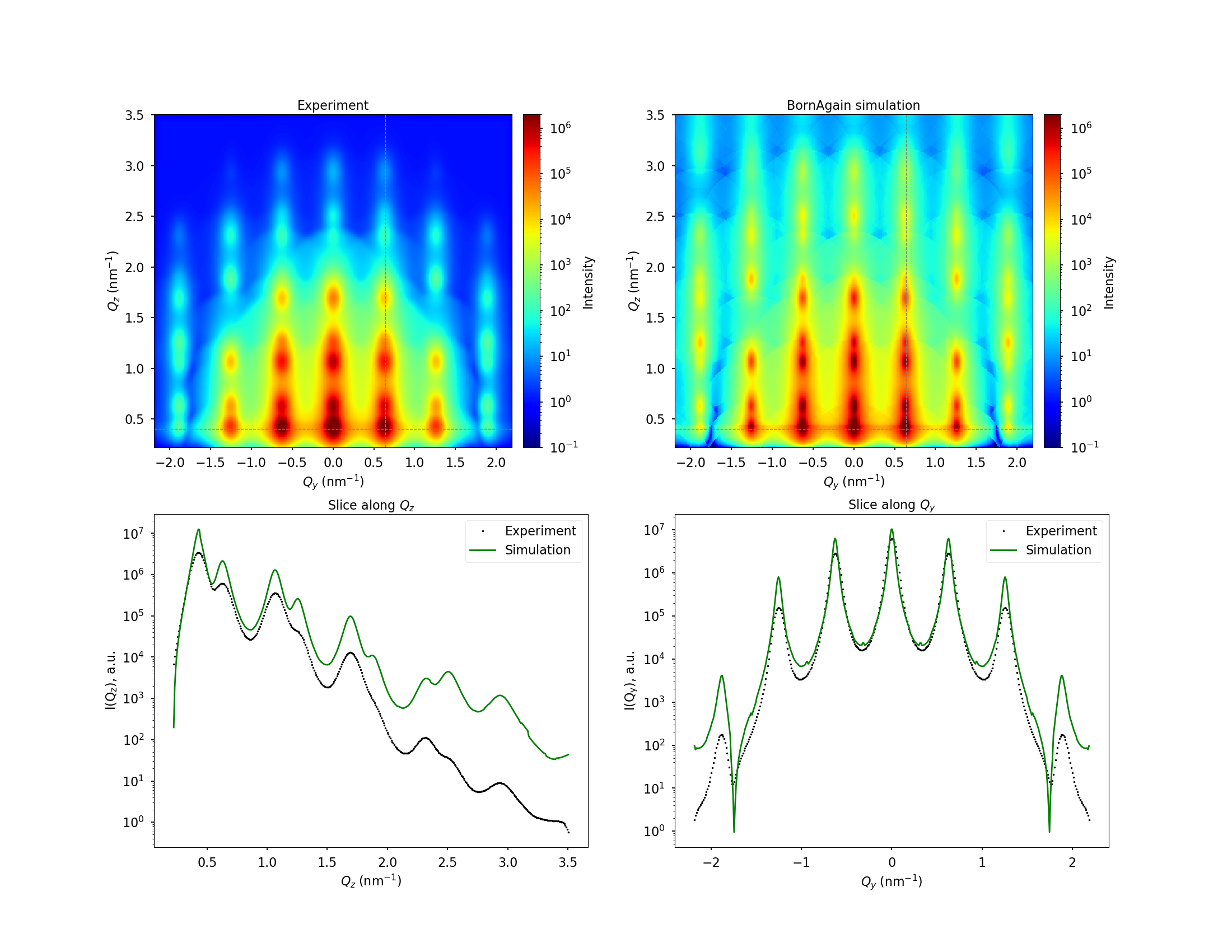
Download files needed to produce this image: