  1
  2
  3
  4
  5
  6
  7
  8
  9
 10
 11
 12
 13
 14
 15
 16
 17
 18
 19
 20
 21
 22
 23
 24
 25
 26
 27
 28
 29
 30
 31
 32
 33
 34
 35
 36
 37
 38
 39
 40
 41
 42
 43
 44
 45
 46
 47
 48
 49
 50
 51
 52
 53
 54
 55
 56
 57
 58
 59
 60
 61
 62
 63
 64
 65
 66
 67
 68
 69
 70
 71
 72
 73
 74
 75
 76
 77
 78
 79
 80
 81
 82
 83
 84
 85
 86
 87
 88
 89
 90
 91
 92
 93
 94
 95
 96
 97
 98
 99
100
101
102
103
104
105
106
107
108
109
110
111
112
113
114
115
116
117
118
119
120
121
122
123
|
#!/usr/bin/env python3
"""
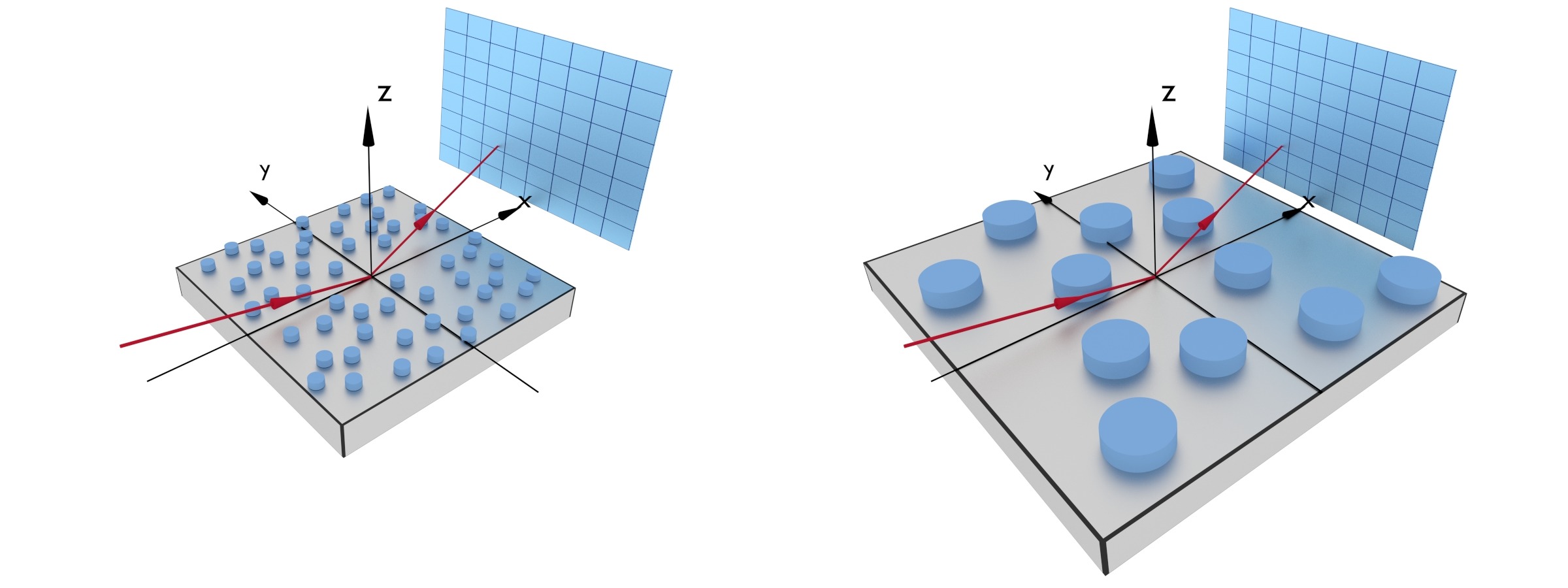
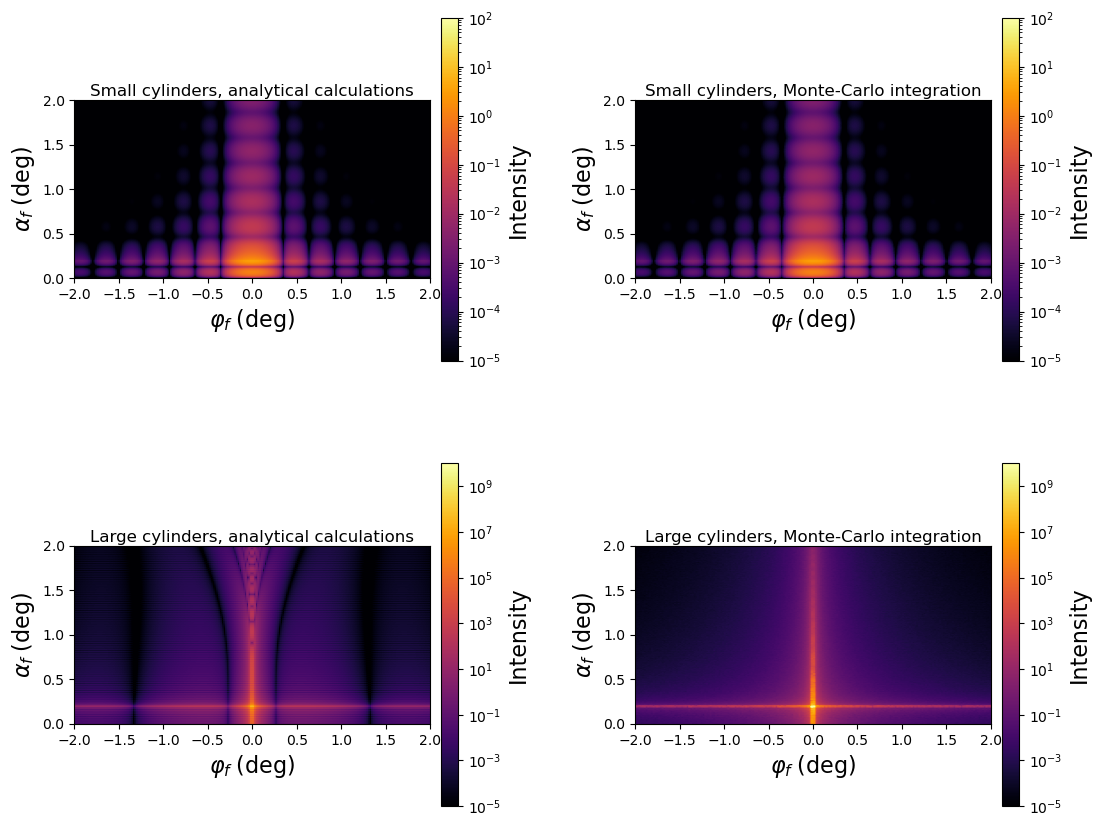
Large cylinders in DWBA.
This example demonstrates that for large particles (~1000nm) the form factor
oscillates rapidly within one detector bin and analytical calculations
(performed for the bin center) give completely wrong intensity pattern.
In this case Monte-Carlo integration over detector bin should be used.
"""
import bornagain as ba
from bornagain import deg, angstrom, nm
import ba_plot
from matplotlib import pyplot as plt
default_cylinder_radius = 10*nm
default_cylinder_height = 20*nm
def get_sample(cylinder_radius, cylinder_height):
# Define materials
m_vacuum = ba.HomogeneousMaterial("Vacuum", 0, 0)
m_substrate = ba.HomogeneousMaterial("Substrate", 6e-6, 2e-8)
m_particle = ba.HomogeneousMaterial("Particle", 6e-4, 2e-8)
# Define particle layout
cylinder_ff = ba.FormFactorCylinder(cylinder_radius, cylinder_height)
cylinder = ba.Particle(m_particle, cylinder_ff)
particle_layout = ba.ParticleLayout()
particle_layout.addParticle(cylinder)
# Define layers
vacuum_layer = ba.Layer(m_vacuum)
vacuum_layer.addLayout(particle_layout)
substrate_layer = ba.Layer(m_substrate)
# Define sample
multi_layer = ba.MultiLayer()
multi_layer.addLayer(vacuum_layer)
multi_layer.addLayer(substrate_layer)
return multi_layer
def get_simulation(sample, integration_flag):
"""
Returns a GISAXS simulation with defined beam and detector.
If integration_flag=True, the simulation will integrate over detector bins.
"""
beam = ba.Beam(1, 1*angstrom, ba.Direction(0.2*deg, 0))
det = ba.SphericalDetector(200, -2*deg, 2*deg, 200, 0, 2*deg)
simulation = ba.GISASSimulation(beam, sample, det)
simulation.getOptions().setMonteCarloIntegration(integration_flag, 50)
if not "__no_terminal__" in globals():
simulation.setTerminalProgressMonitor()
return simulation
def simulate_and_plot():
"""
Run simulation and plot results 4 times: for small and large cylinders,
with and without integration
"""
fig = plt.figure(figsize=(12.80, 10.24))
# conditions to define cylinders scale factor and integration flag
conditions = [{
'title': "Small cylinders, analytical calculations",
'scale': 1,
'integration': False,
'zmin': 1e-5,
'zmax': 1e2
}, {
'title': "Small cylinders, Monte-Carlo integration",
'scale': 1,
'integration': True,
'zmin': 1e-5,
'zmax': 1e2
}, {
'title': "Large cylinders, analytical calculations",
'scale': 100,
'integration': False,
'zmin': 1e-5,
'zmax': 1e10
}, {
'title': "Large cylinders, Monte-Carlo integration",
'scale': 100,
'integration': True,
'zmin': 1e-5,
'zmax': 1e10
}]
# run simulation 4 times and plot results
for i_plot, condition in enumerate(conditions):
scale = condition['scale']
integration_flag = condition['integration']
sample = get_sample(default_cylinder_radius*scale,
default_cylinder_height*scale)
simulation = get_simulation(sample, integration_flag)
simulation.runSimulation()
result = simulation.result()
# plotting results
plt.subplot(2, 2, i_plot + 1)
plt.subplots_adjust(wspace=0.3, hspace=0.3)
zmin = condition['zmin']
zmax = condition['zmax']
ba_plot.plot_colormap(result,
intensity_min=zmin,
intensity_max=zmax)
plt.text(0,
2.1,
conditions[i_plot]['title'],
horizontalalignment='center',
verticalalignment='center',
fontsize=12)
plt.show()
if __name__ == '__main__':
simulate_and_plot()
|