In this example we simulate the scattering from infinite 1D repetition of rectangular patches (rectangular grating). This is done by using the interference function of a 1D lattice together with very long boxes.
length, width, height in the FormFactorBox(length, width, height) constructor correspond to the directions in the $x,y,z$ axes, in that order, so to achieve the desired setup we use the values: length= $10$ nm, width= $10000$ nm, height= $10$ nm.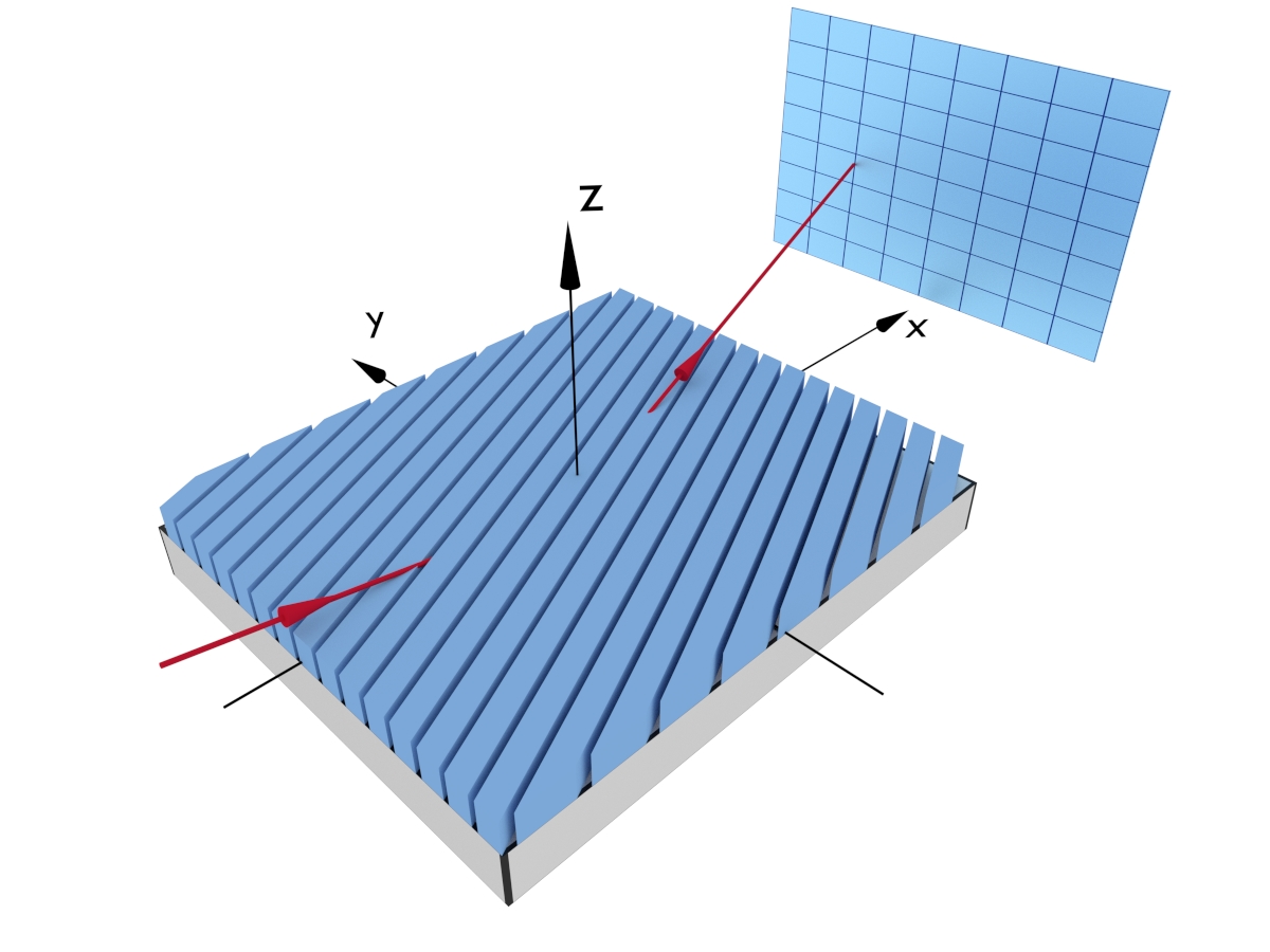
Real-space model
Sketch
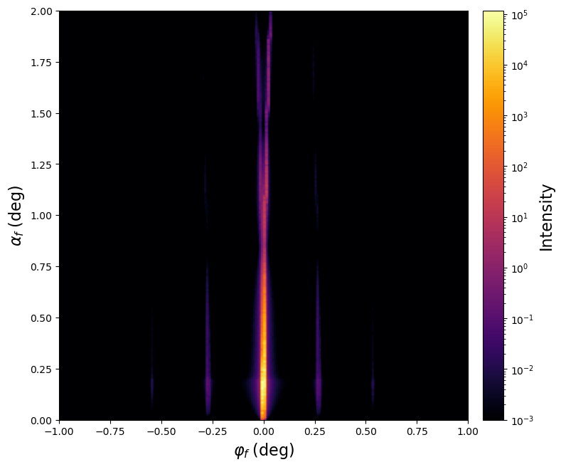
Intensity image
|
|
A one dimensional lattice can be viewed as a chain of particles placed at regular intervals on a single axis. The plot below represents one possible use case, where infinitely long (or very long) boxes are placed at nodes of a 1d lattice to form a grating.

See the BornAgain user manual (Chapter 3.4.1, One Dimensional Lattice) for details about the theory.
The interference function is created using its constructor
InterferenceFunction1DLattice(length, xi)
"""
length : lattice constant, in nanometers
xi : rotation of the lattice with respect to the x-axis, in radians
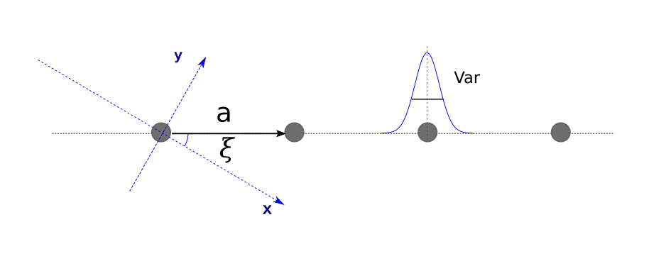
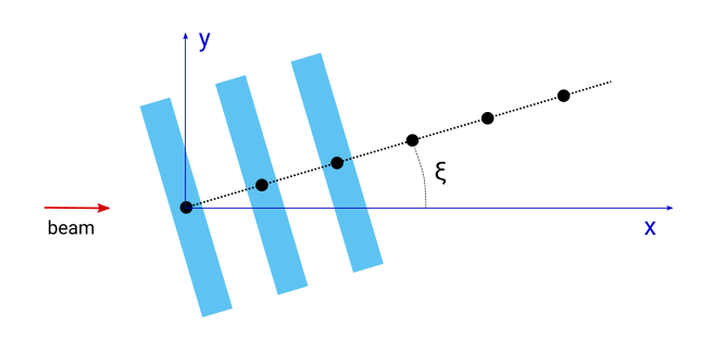
"""Length is the length of the lattice basis vector a expressed in nanometers (see plot below). xi ($\xi$) is the angle defining the lattice orientation. It is taken as the angle between the basis vector of the lattice and the x-axis of the Cartesian coordinate system. It is defined in radians and set to 0 by default.
When the beam azimuthal angle $\varphi_f$ is zero, the beam direction coincides with x-axis. In this case, the $\xi$ angle can be considered as the lattice rotation with respect to the beam.
The position variance parameter Var, as depicted on the top plot, allows to introduce uncertainty for each particle position around the lattice point by applying a corresponding Debye-Waller factor.
It can be set using the setPositionVariance(value) method, where value is given in $nm^2$.
lattice = InterferenceFunction1DLattice(100*nm, 0.0*deg)
lattice.setPositionVariance(0.1)
By default the variance is set to zero.
To account for finite size effects of the lattice, a decay function should be assigned to the interference function. This function encodes the loss of coherent scattering from lattice points with increasing distance between them. The origin of this loss of coherence could be attributed to the coherence length of the beam or to the domain structure of the lattice.
In the picture below a one dimensional lattice is represented in real space as a probability density function for finding a particle at a given coordinate on the x-axis. In the presence of a decay function, this density can be given as $\sum F_{decay}(x)\cdot\delta(x-na)$.
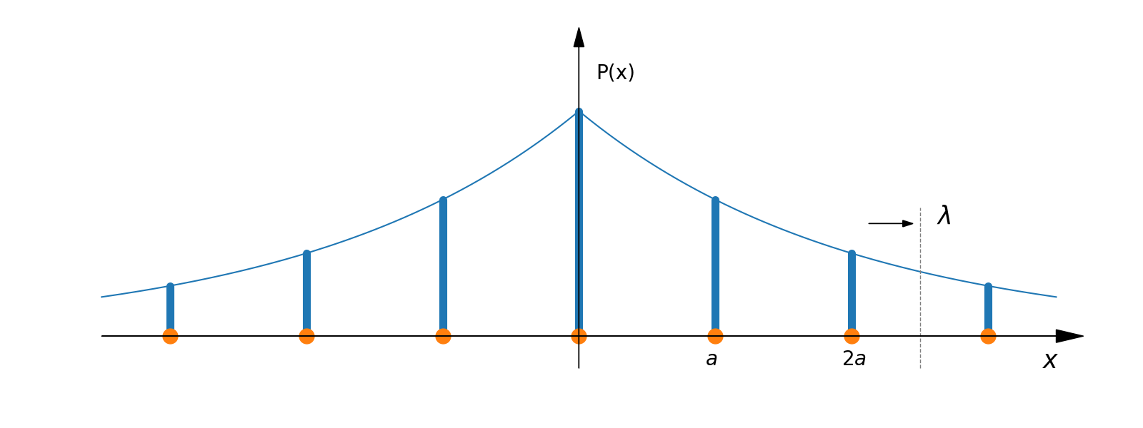
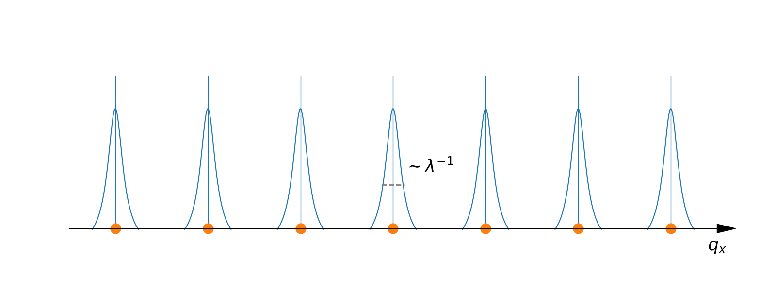
The Fourier transform of this distribution $P(x)$ provides the scattering amplitude in reciprocal space. An exponential decay law in real space with the decay length $\lambda$ will give a Cauchy distribution with characteristic width $1/\lambda$ in reciprocal space, as shown below.
The decay function can be set using the setDecayFunction(decay) method of the 1D interference function.
iff = InterferenceFunction1DLattice(10.0*nm)
iff.setDecayFunction(FTDecayFunction1DCauchy(1000.0*nm))BornAgain supports four types of one-dimensional decay functions.
FTDecayFunction1DCauchy(decay_length)One-dimensional Cauchy decay function in reciprocal space, corresponds to $exp(-|x|/\lambda)$ in real space.
FTDecayFunction1DGauss(decay_length)One-dimensional Gauss decay function in reciprocal space, corresponds to $exp(-x^2/(2*\lambda^2))$ in real space.
FTDecayFunction1DTriangle(decay_length)One-dimensional triangle decay function in reciprocal space, corresponds to $1-|x|/\lambda$, if $|x|<\lambda$, in real space.
FTDecayFunction1DVoigt(decay_length, eta)One-dimensional pseudo-Voigt decay function in reciprocal space, corresponds to $eta*Gauss + (1-eta)*Cauchy$.
The parameter $\lambda$ (decay length) is given in nanometers, it is used to set the characteristic length scale at which loss of coherence takes place. In the case of the pseudo-Voigt distribution an additional dimensionless parameter eta is used to balance between the Gaussian and Cauchy profiles.
During the simulation setup the particle density has to be explicitely specified by the user for correct normalization of overall intensity. This is done by using the ParticleLayout.setParticleDensity(density) method. The density parameter is given here in “number of particles per square nanometer”.
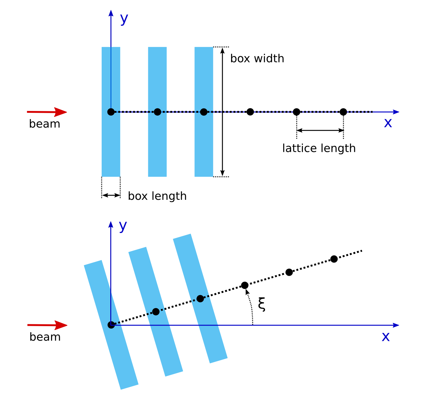
In this paragraph we would like to clarify the relation between the lattice orientation and the orientation of the particles forming the lattice.
For example, we would like to create a grating: a repetition of rectangular patches perpendicular to the beam, as shown on the plot (view from the top of the sample).
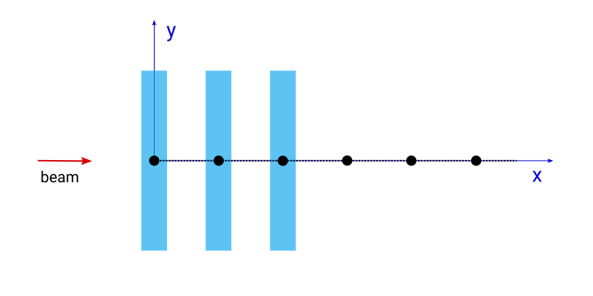
The long side of boxes is aligned along y-axes of the reference plane, the lattice axis coincides with the beam direction, the long side of the boxes is perpendicular to the beam.
To achieve such a setup, the following code should be used.
layout = ba.ParticleLayout()

box = ba.Particle(material, ba.FormFactorBox(10*nm, 1000*nm, 10*nm))
layout.addParticle(box)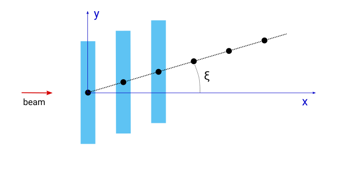
layout.setInterferenceFunction(ba.InterferenceFunction1DLattice(40*nm))If we rotate the lattice by a certain amount, the orientation of the boxes stays the same, but the effective grating period gets smaller. The setup and code are shown below.
box = ba.Particle(material, ba.FormFactorBox(10*nm, 1000*nm, 10*nm))
layout.addParticle(box)
layout.setInterferenceFunction(ba.InterferenceFunction1DLattice(40*nm, 30.0*deg))If we want to preserve the grating period and make our boxes rotate with respect to the beam, a separate rotation should be applied.
box = ba.Particle(material, ba.FormFactorBox(10*nm, 1000*nm, 10*nm))
box.setRotation(ba.RotationZ(30.0*deg))
layout.addParticle(box)
layout.setInterferenceFunction(ba.InterferenceFunction1DLattice(40*nm, 30.0*deg))To Initialize InterferenceFunction1DLattice in the graphical user interface, the corresponding object has to be connected with ParticleLayout and the corresponding parameters (lattice length, rotation and parameters of decay function) have to be adjusted in the property editor.
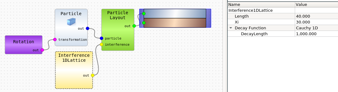
In the given example, an additional rotation module is attached to the box to provide a rotation around the z-axis and achieve the configuration of Setup 3 from the example above.