1
  2
  3
  4
  5
  6
  7
  8
  9
 10
 11
 12
 13
 14
 15
 16
 17
 18
 19
 20
 21
 22
 23
 24
 25
 26
 27
 28
 29
 30
 31
 32
 33
 34
 35
 36
 37
 38
 39
 40
 41
 42
 43
 44
 45
 46
 47
 48
 49
 50
 51
 52
 53
 54
 55
 56
 57
 58
 59
 60
 61
 62
 63
 64
 65
 66
 67
 68
 69
 70
 71
 72
 73
 74
 75
 76
 77
 78
 79
 80
 81
 82
 83
 84
 85
 86
 87
 88
 89
 90
 91
 92
 93
 94
 95
 96
 97
 98
 99
100
101
102
103
104
105
106
107
108
109
110
111
112
113
114
115
116
117
118
119
120
121
122
123
124
125
126
127
128
129
130
131
132
133
134
135
136
137
138
139
140
141
142
143
144
145
146
147
148
149
150
151
152
153
154
155
156
157
158
159
160
161
162
163
164
165
166
167
168
169
170

#!/usr/bin/env python3
"""
Extended example for simulation results treatment (cropping, slicing, exporting)
The standard "Cylinders in DWBA" sample is used to setup the simulation.
"""
import math
import random
import bornagain as ba
from bornagain import angstrom, deg, nm, nm2, kvector_t
import ba_plot
from matplotlib import pyplot as plt
from matplotlib import rcParams


def get_sample():
    """
    Returns a sample with uncorrelated cylinders on a substrate.
    """

    # Define materials
    material_Particle = ba.HomogeneousMaterial("Particle", 0.0006, 2e-08)
    material_Substrate = ba.HomogeneousMaterial("Substrate", 6e-06, 2e-08)
    material_Vacuum = ba.HomogeneousMaterial("Vacuum", 0, 0)

    # Define form factors
    ff = ba.FormFactorCylinder(5*nm, 5*nm)

    # Define particles
    particle = ba.Particle(material_Particle, ff)

    # Define particle layouts
    layout = ba.ParticleLayout()
    layout.addParticle(particle)
    layout.setTotalParticleSurfaceDensity(0.01)

    # Define layers
    layer_1 = ba.Layer(material_Vacuum)
    layer_1.addLayout(layout)
    layer_2 = ba.Layer(material_Substrate)

    # Define sample
    sample = ba.MultiLayer()
    sample.addLayer(layer_1)
    sample.addLayer(layer_2)

    return sample


def get_simulation(sample):
    """
    Returns a GISAXS simulation with beam and detector defined.
    """
    beam = ba.Beam(1e5, 1*angstrom, ba.Direction(0.2*deg, 0))
    det = ba.SphericalDetector(201, -2*deg, 2*deg, 201, 0, 2*deg)
    simulation = ba.GISASSimulation(beam, sample, det)
    return simulation


def get_noisy_image(hist):
    """
    Returns clone of input histogram filled with additional noise
    """
    result = hist.clone()
    noise_factor = 2.0
    for i in range(0, result.getTotalNumberOfBins()):
        amplitude = result.binContent(i)
        sigma = noise_factor*math.sqrt(amplitude)
        noisy_amplitude = random.gauss(amplitude, sigma)
        result.setBinContent(i, noisy_amplitude)
    return result


def plot_histogram(hist, **kwargs):
    ba.plot_histogram(hist,
                      xlabel=r'$\varphi_f ^{\circ}$',
                      ylabel=r'$\alpha_f ^{\circ}$',
                      zlabel="",
                      **kwargs)


def get_relative_difference(hist):
    """
    Creates noisy histogram made of original histogram,
    then creates and plots a relative difference histogram: (noisy-hist)/hist
    """
    noisy = get_noisy_image(hist)
    return noisy.relativeDifferenceHistogram(hist)


def plot_slices(hist):
    """
    Plot 1D slices along y-axis at certain x-axis values.
    """
    noisy = get_noisy_image(hist)

    # projection along Y, slice at fixed x-value
    proj1 = noisy.projectionY(0)
    plt.semilogy(proj1.binCenters(),
                 proj1.binValues(),
                 label=r'$\phi=0.0^{\circ}$')

    # projection along Y, slice at fixed x-value
    proj2 = noisy.projectionY(0.5)  # slice at fixed value
    plt.semilogy(proj2.binCenters(),
                 proj2.binValues(),
                 label=r'$\phi=0.5^{\circ}$')

    # projection along Y for all X values between [xlow, xup], averaged
    proj3 = noisy.projectionY(0.41, 0.59)
    plt.semilogy(proj3.binCenters(),
                 proj3.array(ba.IHistogram.AVERAGE),
                 label=r'$<\phi>=0.5^{\circ}$')

    plt.xlim(proj1.getXmin(), proj1.getXmax())
    plt.ylim(proj2.getMinimum(), proj1.getMaximum()*10)
    plt.xlabel(r'$\alpha_f ^{\circ}$', fontsize=16)
    plt.legend(loc='upper right')
    plt.tight_layout()


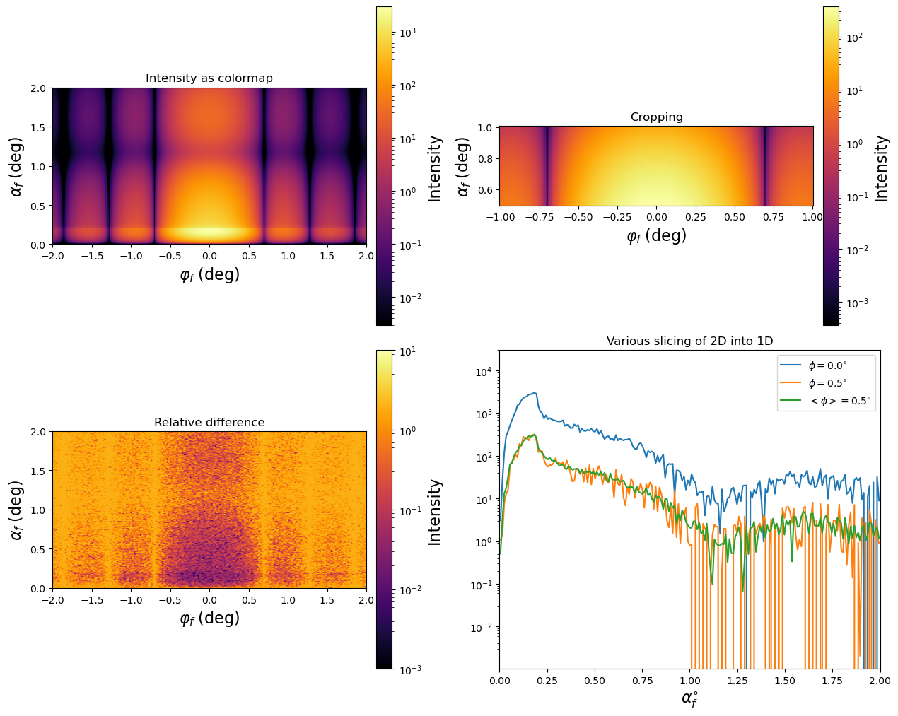
def plot(hist):
    """
    Runs different plotting functions one by one
    to demonstrate trivial data presentation tasks.
    """
    plt.figure(figsize=(12.80, 10.24))

    plt.subplot(2, 2, 1)
    ba_plot.plot_histogram(hist)
    plt.title("Intensity as colormap")

    plt.subplot(2, 2, 2)
    crop = hist.crop(-1, 0.5, 1, 1)
    ba_plot.plot_histogram(crop)
    plt.title("Cropping")

    plt.subplot(2, 2, 3)
    reldiff = get_relative_difference(hist)
    ba_plot.plot_histogram(reldiff, intensity_min=1e-03, intensity_max=10)
    plt.title("Relative difference")

    plt.subplot(2, 2, 4)
    plot_slices(hist)
    plt.title("Various slicing of 2D into 1D")

    # save to file
    # result.save("result.int")
    # result.save("result.tif")
    # result.save("result.txt")
    # result.save("result.int.gz")
    # result.save("result.tif.gz")
    # result.save("result.txt.gz")
    # result.save("result.int.bz2")
    # result.save("result.tif.bz2")
    # result.save("result.txt.bz2")

    plt.tight_layout()
    plt.show()


def simulate_and_plot():
    sample = get_sample()
    simulation = get_simulation(sample)
    simulation.runSimulation()
    hist = simulation.result().histogram2d()
    plot(hist)


if __name__ == '__main__':
    simulate_and_plot()