Polarized specular reflectometry with non-perfect polarizer and analyzer

In this example, we show how to perform a specular reflectometry simulation with polarized neutrons and both a non-perfect polarizer as well as analyzer. The example is inspired by and performed with parameters close to the ones in the paper by Devishvili et al.. This example is a saturated iron film on top of a MgO substrate. On top of the iron layer is a thin Pd cap layer.

We don’t explain the whole script in detail here, it combines all concepts that were introduced before in the polarized reflectometry section. Instrument resolution is simulated as explained in the ToF - Resolution effects example. Furthermore, a constant background is added:

simulation.setBackground( ba.ConstantBackground( 1e-7 ) )

For a more detailed explanation we refer to the example on adding a constant background.

The values for the efficiency of the polarizer and analyzer are taken from the above mentioned paper by Devishvili et al.:

polarizer_efficiency = 0.986
analyzer_efficiency  = 0.970

These values are used to initialize the polarizer and analyzer:

simulation.setBeamPolarization(polarization * polarizer_efficiency)
simulation.setAnalyzerProperties(analyzer, analyzer_efficiency, 0.5)

This setup is then utilized to simulate the four reflectivity channels

results_pp = run_simulation(polarization = ba.kvector_t(0, 1, 0), 
                            analyzer     = ba.kvector_t(0, 1, 0), 
                            polarizer_efficiency = polarizer_efficiency,
                            analyzer_efficiency  = analyzer_efficiency )
results_mm = run_simulation(polarization = ba.kvector_t(0, -1, 0), 
                            analyzer     = ba.kvector_t(0, -1, 0), 
                            polarizer_efficiency = polarizer_efficiency,
                            analyzer_efficiency  = analyzer_efficiency )

results_pm = run_simulation(polarization = ba.kvector_t(0,  1, 0), 
                            analyzer     = ba.kvector_t(0, -1, 0), 
                            polarizer_efficiency = polarizer_efficiency,
                            analyzer_efficiency  = analyzer_efficiency )
results_mp = run_simulation(polarization = ba.kvector_t(0, -1, 0), 
                            analyzer     = ba.kvector_t(0,  1, 0), 
                            polarizer_efficiency = polarizer_efficiency,
                            analyzer_efficiency  = analyzer_efficiency )

The computed reflectivity looks like this:
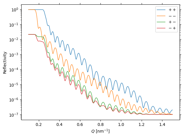
Reflectivity

Due to the different values for the polarizer and analyzer efficiency, we obtain different reflectivity curves for the two spin-flip channels. As one can verify, these results are in good agreement with the measurement as well as the simulations presented by Devishvili et al.

Here is the complete example:

  1
  2
  3
  4
  5
  6
  7
  8
  9
 10
 11
 12
 13
 14
 15
 16
 17
 18
 19
 20
 21
 22
 23
 24
 25
 26
 27
 28
 29
 30
 31
 32
 33
 34
 35
 36
 37
 38
 39
 40
 41
 42
 43
 44
 45
 46
 47
 48
 49
 50
 51
 52
 53
 54
 55
 56
 57
 58
 59
 60
 61
 62
 63
 64
 65
 66
 67
 68
 69
 70
 71
 72
 73
 74
 75
 76
 77
 78
 79
 80
 81
 82
 83
 84
 85
 86
 87
 88
 89
 90
 91
 92
 93
 94
 95
 96
 97
 98
 99
100
101
102
103
104
105
106
107
108
109
110
111
112
113
114
115
116
117
118
119
120
121
122
123
124
125
126
127
128
129
130
131
132
133
134
135
136
137
138
139
#!/usr/bin/env python3
"""
An example that shows how to simulate
a non-perfect polarizer and analyzer
following Devishvili et al., Rev. Sci. Instrum. 84, 025112 (2013)
"""
import numpy
import matplotlib.pyplot as plt

import bornagain as ba
from bornagain import deg, angstrom

sldFe = (8.0241e-06, 6.0448e-10)
sldPd = (4.0099e-6, 1.3019e-09)
sldMgO = (5.9803e-06, 9.3996e-12)

magnetizationMagnitude = 1.6e6
angle = 0
magnetizationVector = ba.kvector_t(
    magnetizationMagnitude*numpy.sin(angle*deg),
    magnetizationMagnitude*numpy.cos(angle*deg), 0)


def get_sample(*, magnetization=magnetizationVector):
    """
    Define sample and returns it
    """

    # create materials
    mat_vacuum = ba.MaterialBySLD("Vacuum", 0, 0)
    mat_Pd = ba.MaterialBySLD("Pd", *sldPd)
    mat_Fe = ba.MaterialBySLD("Fe", *sldFe, magnetizationVector)
    mat_substrate = ba.MaterialBySLD("MgO", *sldMgO)

    # create layers
    layer_vacuum = ba.Layer(mat_vacuum)
    layer_Pd = ba.Layer(mat_Pd, 120*angstrom)
    layer_Fe = ba.Layer(mat_Fe, 1000*angstrom)
    layer_substrate = ba.Layer(mat_substrate)

    roughness = ba.LayerRoughness()
    roughness.setSigma(20*angstrom)

    # create sample
    multi_layer = ba.MultiLayer()

    multi_layer.addLayer(layer_vacuum)
    multi_layer.addLayerWithTopRoughness(layer_Pd, roughness)
    multi_layer.addLayerWithTopRoughness(layer_Fe, roughness)
    multi_layer.addLayerWithTopRoughness(layer_substrate, roughness)

    return multi_layer


def get_simulation(sample, scan_size=1500):
    """
    Defines and returns a specular simulation.
    """
    simulation = ba.SpecularSimulation()
    qzs = numpy.linspace(0.1, 1.5, scan_size)

    n_sig = 4.0
    n_samples = 25
    distr = ba.RangedDistributionGaussian(n_samples, n_sig)

    scan = ba.QSpecScan(qzs)
    scan.setAbsoluteQResolution(distr, 0.008)

    simulation.setScan(scan)
    simulation.setSample(sample)
    return simulation


def run_simulation(*,
                   polarization=ba.kvector_t(0, 1, 0),
                   polarizer_efficiency=1,
                   analyzer=ba.kvector_t(0, 1, 0),
                   analyzer_efficiency=1):
    """
    Runs simulation and returns its result.
    """
    sample = get_sample()
    simulation = get_simulation(sample)

    simulation.beam().setPolarization(polarization*polarizer_efficiency)
    simulation.detector().setAnalyzerProperties(analyzer,
                                                analyzer_efficiency, 0.5)

    simulation.setBackground(ba.ConstantBackground(1e-7))

    simulation.runSimulation()
    return simulation.result()


def plot(data, labels):

    plt.figure()
    for d, l in zip(data, labels):
        plt.semilogy(numpy.array(d.axis(ba.Axes.QSPACE)),
                     d.array(ba.Axes.QSPACE),
                     label=l,
                     linewidth=1)

    plt.legend(loc='upper right')
    plt.gca().yaxis.set_ticks_position('both')
    plt.gca().xaxis.set_ticks_position('both')

    plt.xlabel("$Q$ [nm${}^{-1}$]")
    plt.ylabel("Reflectivity")

    plt.tight_layout()
    plt.show()


if __name__ == '__main__':

    polarizer_efficiency = 0.986
    analyzer_efficiency = 0.970

    results_pp = run_simulation(polarization=ba.kvector_t(0, 1, 0),
                                analyzer=ba.kvector_t(0, 1, 0),
                                polarizer_efficiency=polarizer_efficiency,
                                analyzer_efficiency=analyzer_efficiency)
    results_mm = run_simulation(polarization=ba.kvector_t(0, -1, 0),
                                analyzer=ba.kvector_t(0, -1, 0),
                                polarizer_efficiency=polarizer_efficiency,
                                analyzer_efficiency=analyzer_efficiency)

    results_pm = run_simulation(polarization=ba.kvector_t(0, 1, 0),
                                analyzer=ba.kvector_t(0, -1, 0),
                                polarizer_efficiency=polarizer_efficiency,
                                analyzer_efficiency=analyzer_efficiency)
    results_mp = run_simulation(polarization=ba.kvector_t(0, -1, 0),
                                analyzer=ba.kvector_t(0, 1, 0),
                                polarizer_efficiency=polarizer_efficiency,
                                analyzer_efficiency=analyzer_efficiency)

    plot([results_pp, results_mm, results_pm, results_mp],
         ["$++$", "$--$", "$+-$", "$-+$"])
PolarizedNonperfectAnalyzerPolarizer.py