Scattering from monodisperse cylinders distributed along a two-dimensional square paracrystal.
Note:
A damping length is used to introduce finite size effects by applying a multiplicative coefficient equal to $exp \left(-\frac{peak\_distance}{damping\_length}\right)$ to the Fourier transform of the probability densities. $damping\_length$ is equal to $0$ by default and, in this case, no correction is applied.
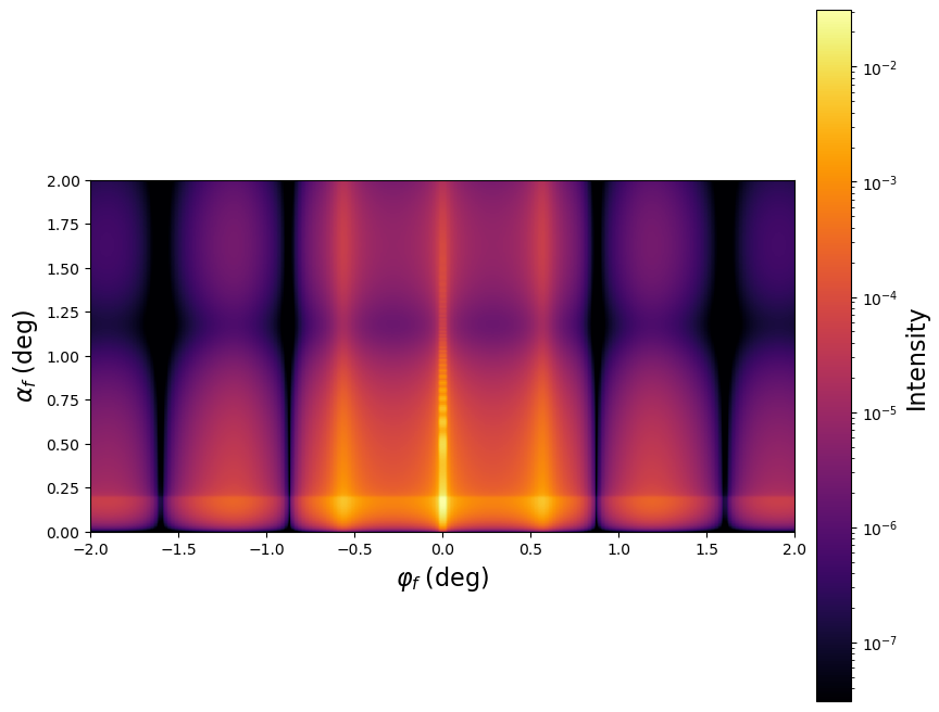
Intensity image
|
|
Similarly to the 2D interference function, the 2D paracrystal is used to model the scattering from particles positioned at some regular intervals on a plane. However, the 2D paracrystal model posesses only short range order. The disorder is cumulative at further distance.
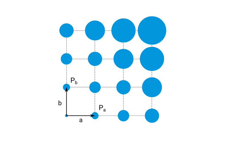
The plot above represents a schematic view of the 2D paracrystal. Each circle on the plot represents an area where the probability to find a particle, given a particle at the origin, is above some arbitrary threshold. The growing size of the areas emphasizes the fact that our knowledge about the next neighbor’s location decreases with the distance to the origin.
The two-dimensional paracrystal model in BornAgain is implemented as a simple convolution of two one-dimensional paracrystals along the lattice basis directions.
The user defines lattice constants and provides probability distributions of the first neighbor along each of two lattice axes. On the plot above, these distributions are marked $P_a$ and $P_b$ and are represented by two circles of same size. The probability distributions of finding other particles along lattice vectors will be deduced from accumulating position uncertainties of previous particles towards the origin. In the general case, $P_a$ and $P_b$ can have different sizes and have different orientation with respect to the lattice axes.
The BornAgain user manual (Chapter 3.5, Paracrystal) details the theoretical model and gives some links to the literature.
The interference is created using its constructor.
InterferenceFunction2DParaCrystal(length1, length2, alpha, xi = 0.0, damping_length = 0.0)
"""
length1, length2 : lengths of the lattice cell, in nanometers
alpha : angle between lattice vectors, in radians
xi : rotation angle of the lattice with respect to the x-axis, in radians
damping_length : The damping (coherence) length of the paracrystal in nanometers.
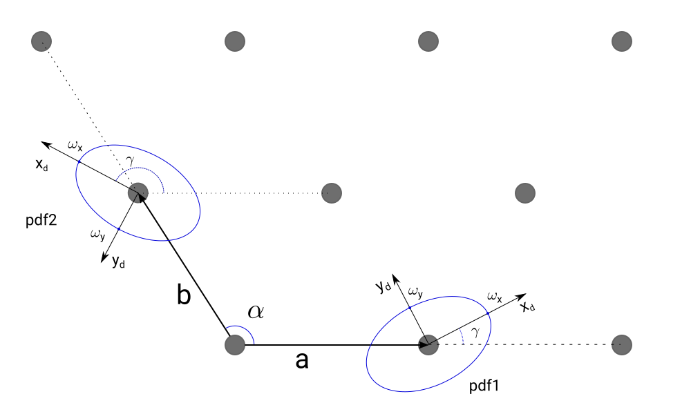
"""length1 and length2 are lengths of lattice vectors $a$, $b$ expressed in nanometers (see plot below). alpha is the angle between the lattice basis vectors $a$, $b$ in direct space (in radians). xi is the angle defining the lattice orientation . It is taken as the angle between the first lattice basis vector and the x-axis of the reference cartesian frame. It is expressed in radians and set to 0 by default.
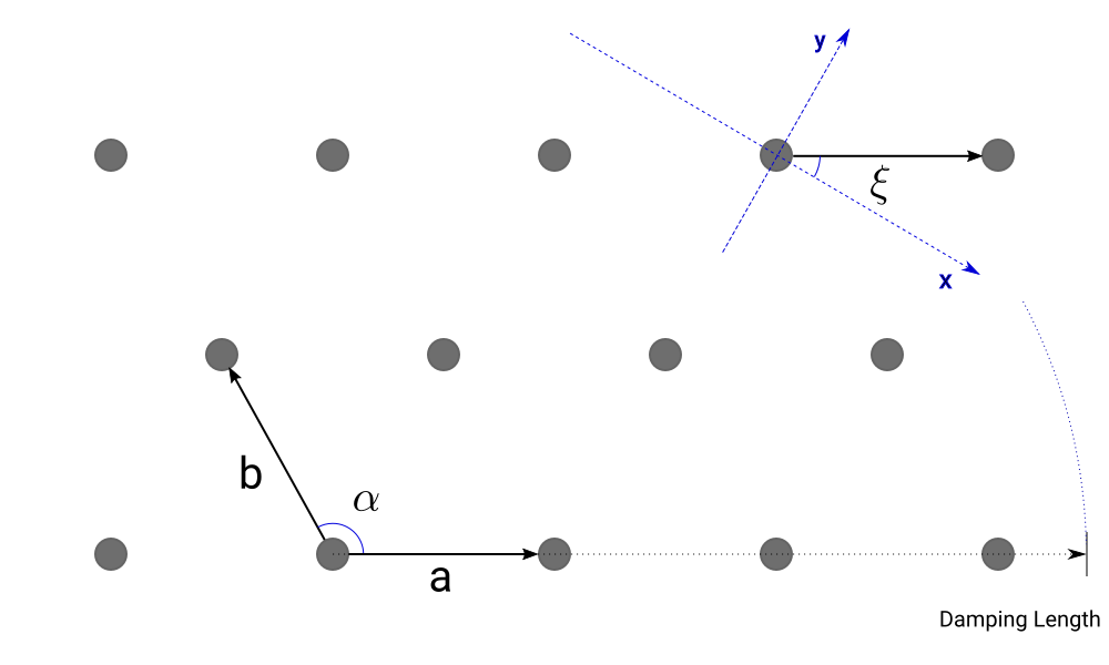
When the beam azimuthal angle $\varphi_f$ is zero, the beam direction coincides with x-axis of the reference frame, so angle $\xi$ can be considered as the lattice rotation with respect to the beam.
The parameter damping_length is used to introduce finite size effects by applying a multiplicative coefficient equal to exp(-lattice_constant/damping_length) to the Fourier transform of the probability density of a nearest neighbor. damping_length is equal to 0 by default and, in this case, no correction is applied. On the plot above the damping length is provisionally depicted as an area contributing to the scattering.
To account for next neighbor position uncertainty a probability distribution should be assigned to the interference function. This is done using the setProbabilityDistribution(pdf1, pdf2) method of the 2d paracrystal object, with pdf1,2 related to each main axis of the paracrystal.
The probability distribution is parameterized with its type, size and orientation with respect to the lattice vector. $x_d$, $y_d$ on the plot below represent an orthonormal coordinate system of the distribution in real space which is rotated by the angle gamma with respect to the lattice vector. pdf1 is defined for lattice vector $a$, and pdf2 for lattice vector $b$.
The following PDF distributions are available
# Fourier transform of Cauchy-Lorentzian
FTDistribution2DCauchy(omega_x, omega_y, delta=0)

# Fourier transform of a Gaussian
FTDistribution2DGauss(omega_x, omega_y, delta=0)

# Fourier transform of a gate distribution
FTDistribution2DGate(omega_x, omega_y, delta=0)

# Fourier transform of a triangle distribution
FTDistribution2DTriangle(omega_x, omega_y, delta=0)

# Fourier transform of a pseudo-Voigt distribution: eta*Gauss + (1-eta)*Cauchy
FTDistribution2DVoigt(omega_x, omega_y, eta, delta=0)
All distributions have parameters
omega_x  : half-width of the distribution along its x-axis in nanometers
omega_y  : half-width of the distribution along its y-axis in nanometers
gamma    : angle in direct space between first lattice vector and x-axis of the distribution
In the case of the Voigt distribution, an additional dimensionless parameter eta is used to balance between Gaussian and Cauchy profiles.
The interference function of a 2D paracrystal provides a way to calculate the scattering from a finite portion of the paracrystal using the setDomainSize(size1, size2) method. Here size1, size2 are given in nanometers and represent the sizes of the coherence domains in the first and second lattice directions.
The resulting behaviour is similar to the case when damping_length is used (the difference in computation is explained in the user manual). In the code snippet below, the paracrystal is created without specifying the damping_length (i.e. to rely on its default value 0), and then the setDomainSize method is used to introduce the alternative mechanism for finite size corrections.
iff = InterferenceFunction2DParacrystal(20.0*nm, 20.0*nm, 90.0*deg)
iff.setProbabilityDistribution(FTDistribution2DCauchy(30.0*nm), FTDistribution2DCauchy(30.0*nm))
iff.setDomainSize(10000*nm, 10000*nm)Two convenience functions allow to create square and hexagonal paracrystals without the need to specify the second lattice vector and the lattice angle.
# interference function of a square lattice
InterferenceFunction2DParaCrystal.createSquare(lattice_constant, damping_length=0, domain_size1=0, domain_size2=0)

# interference function of a hexagonal lattice
InterferenceFunction2DLattice.createHexagonal(lattice_constant, damping_length=0, domain_size1=0, domain_size2=0)The computational kernel provides an automatic calculation of particle densities using the parameters of the 2D lattice. This means, that the user’s settings of particle densities via the ParticleLayout.setParticleDensity() method (which is a required step in the case of a radial paracrystal interference function) is ignored.
Averaging over lattice rotation angle.
The paracrystal 2D interference function can be averaged over all azimuthal angles $\xi$ using the setIntegrationOverXi(True) method. In this case the initial lattice rotation angle $\xi$, if set, will be ingnored and numeric integration will be performed for $\xi$ in the range 0, 360 degrees. Averaging provides a convenient way of getting an isotropic interference function for the cost of bigger computational time.
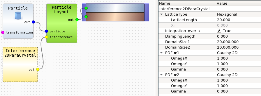
To initialize the InterferenceFunction2DParaCrystal in the graphical user interface, the corresponding object has to be connected with ParticleLayout and its parameters (lattice length, angles, PDF function parameters) adjusted in the property editor.