A RectangularDetector object in BornAgain is used to represent a two dimensional neutron/x-ray detector. The following sections provide details on this type of detector:
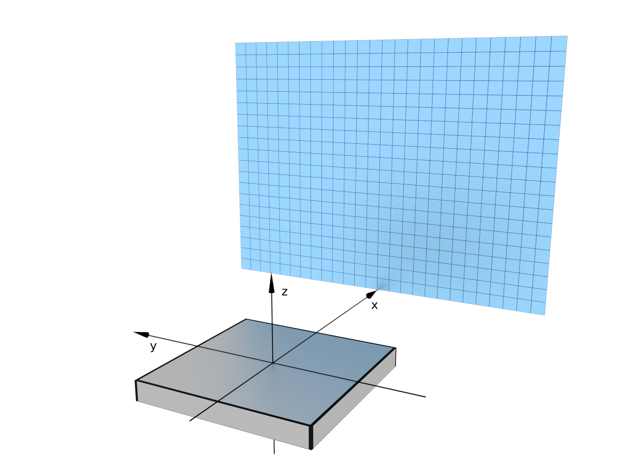
A RectangularDetector has a plane rectangular shape, a total given width and height and a given amount of pixels. The detector plane can placed in an arbitrary position and orientation with respect to the sample position.
Note
Real experimental setups vary significantly from one GISAS instrument to another. Different conventions for representing the space coordinates, a range of detector’s positions/orientations and different detector’s alignment techniques make the creation of a universal detector API quite challenging. The BornAgain detector API is generic enough to be able to cope with all the aforementioned differences and, hopefully, is simple enough to let the user quickly setup his specific case.
BornAgain’s RectangularDetector is initialized using its constructor
RectangularDetector(nxbins, width, nybins, height)
"""
Constructs rectangular planar detector

nxbins : Number of bins (pixels) in x-direction
width  : Width of the detector in mm along x-direction
nybins : Number of bins (pixels) in y-direction
height : Height of the detector in mm along y-direction
"""
The local detector coordinate system is defined in such a way, that its origin coincides with the lower left corner of the rectangle. For example, the following code snippet will create a rectangular detector with a total number of pixels equal to $10 \cdot 9=90$ and with a pixel size equal to $200 mm \cdot 180 mm =36\cdot 10^3 mm^2$.
detector = RectangularDetector(10, 200.0, 9, 180.0)
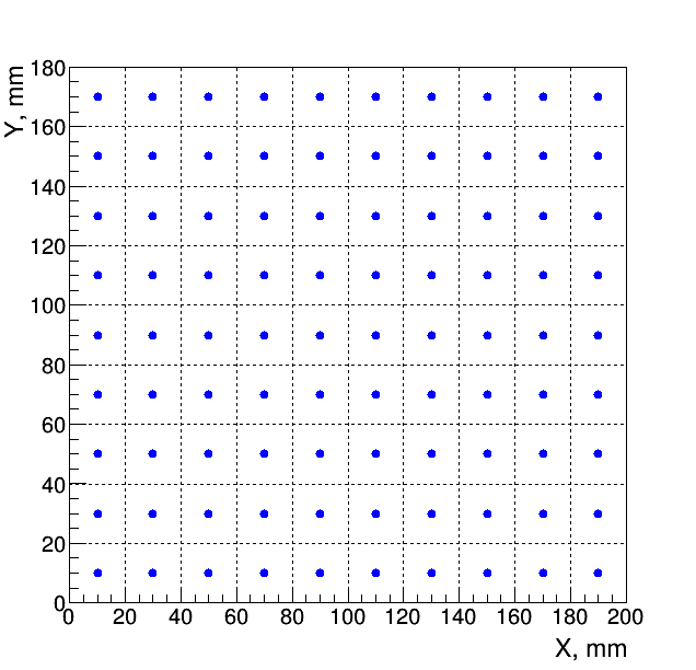
Here, the vertical and horizontal lines denote the bin boundaries while the blue markers show the bin centers. During a simulation, the bin intensity will be calculated for values of $\varphi_f$ and $\alpha_f$ corresponding to the bin centers and then normalized to the bin area.
Note
GISASSimulation has a special setting to calculate the intensity in a bin as the 2D integral along the detector bin area. This mode will be explained elsewhere.
The position and the orientation of the detector can be defined in a generic way using the following parameters:
(u0, v0) of intersection of the normal vector n and the detector plane, expressed in local detector coordinates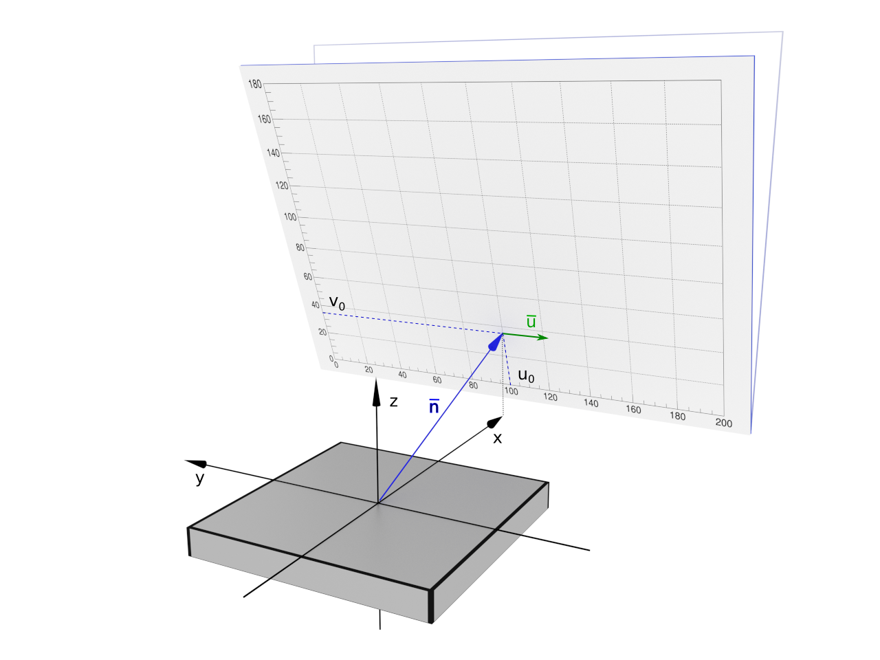
In the plot above, the detector is inclined towards the sample by an angle of 20 degrees.
The position is defined using the RectangularDetector::setPosition method as follows
setPosition(normal, u0, v0, direction=kvector_t(0, -1, 0))
"""
Sets position of rectangular detector
normal   : Vector in sample coordinate system, normal to the detector plane,
           pointing from the sample origin to the detector plane
u0       : x-coordinate of point of intersection of normal vector and detector plane,
           expressed in local detector coordinates
v0       : y-coordinate of point of intersection of normal vector and detector plane,
           expressed in local detector coordinates
direction: direction of detector u-axis with respect to the sample coordinate system
"""
Please note, that the direction vector u is set by default to (0.0, -1.0, 0.0) which corresponds to the detector u-axis pointing to the right, as shown in the plot above (green arrow on the detector plane). This value should not be changed, unless the user has to deal with a rotation of the detector around the normal vector n.
In the following, we will show how to set the detector’s parameters for the three most common cases in GISAS experimental setups:
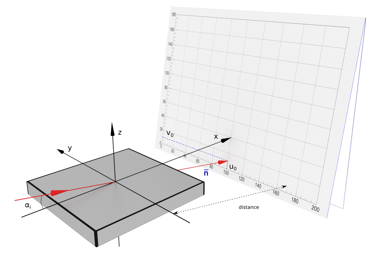
In this case the normal vector n coincides with the x-axis of the sample coordinate system and the length of the vector is equal to the detector distance. The detector’s local coordinates (u0, v0) denote the point where the sample x-axis crosses the detector plane.
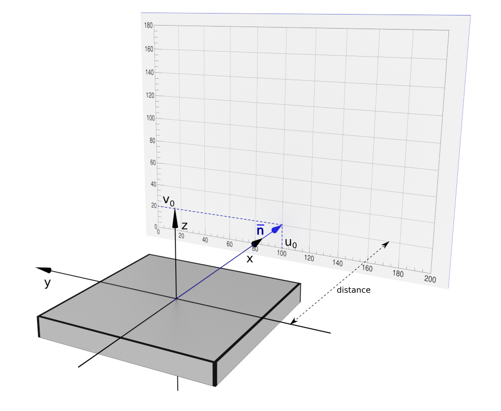
The following code demonstrates the creation of the detector shown in the plot. Please note, that the values of the parameters are given only as an example and do not reflect the relative proportions in the plot.
nxbins, nybins = 10, 9
width, height = 200.0, 180.0
distance = 2000.0
u0, v0 = 100.0, 20.0

detector = RectangularDetector(nxbins, width, nybins, height)
detector.setPosition(kvector_t(distance, 0.0, 0.0), u0, v0)

simulation = GISASSimulation()
simulation.setDetector(detector)
The convenience method RectangularDetector::setPerpendicularToSampleX can be used to achieve the same setup:
detector = RectangularDetector(nxbins, width, nybins, height)
detector.setPerpendicularToSampleX(distance, u0, v0)
In this case the normal vector n coincides with the beam direction. The length of the vector is equal to the sample-detector distance. The detector local coordinates (u0, v0) again denote the point where the direct beam hits the detector plane.
The normal vector n can be easily calculated from the beam inclination angle $\alpha_i$.
width, height = 200.0, 180.0
distance = 2000.0
u0, v0 = 100.0, 10.0
alpha_i = 0.2*deg

detector = RectangularDetector(nxbins, width, nybins, height)
normal = kvector_t(distance*cos(alpha_i), 0.0, -1.0*distance*sin(alpha_i)))
detector.setPosition(normal, u0, v0)

simulation = GISASSimulation()
simulation.setDetector(detector)
The convenience method RectangularDetector::setPerpendicularToDirectBeam can be used to simplify this setup:
detector = RectangularDetector(nxbins, width, nybins, height)
detector.setPerpendicularToDirectBeam(distance, u0, v0)
In this case, the GISASSimulation will calculate the normal vector n during runtime, depending from the beam angle settings.
In this case the normal vector n coincides with the reflected beam direction. The length of the vector is equal to the sample-detector distance. The detector local coordinates (u0, v0) denote the point where the reflected beam hits the detector plane.
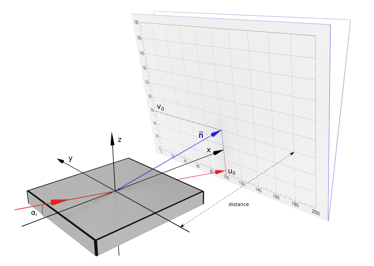
The normal vector n can be easily calculated from the beam inclination angle $\alpha_i$.
distance = 2000.0
u0, v0 = 100.0, 60.0
alpha_i = 0.2*deg

detector = RectangularDetector(nxbins, width, nybins, height)
normal = kvector_t(distance*cos(alpha_i), 0.0, distance*sin(alpha_i)))
detector.setPosition(normal, u0, v0)

simulation = GISASSimulation()
simulation.setDetector(detector)
The convenience method RectangularDetector::setPerpendicularToReflectedBeam can be used to simplify this setup:
detector = RectangularDetector(nxbins, width, nybins, height)
detector.setPerpendicularToReflectedBeam(distance, u0, v0)
In this case, the GISASSimulation will calculate the normal vector n during runtime, depending on the beam angle settings.
All methods described above to initialize a detector, use the coordinates (u0, v0) - the coordinates of the point where the normal vector n hits the detector plane, expressed in the local detector coordinates.
In the case of a detector perpendicular to the direct beam, these coordinates, naturally, coincide with the point where the direct beam hits the detector. For a detector perpendicular to the reflected beam, these coordinates coincide with the point where the reflected beam hits the detector.
If the coordinates of the reflected beam in the detector plane are not known, a convenience method RectangularDetector::setDirectBeamPosition can be used. For example, the following combination is possible:
detector = RectangularDetector(nxbins, width, nybins, height)
detector.setPerpendicularToReflectedBeam(distance)  # note that (u0,v0) are omitted
direct_beam_xpos = 100.0
direct_beam_ypos = 5.0
detector.setDirectBeamPosition(direct_beam_xpos, direct_beam_ypos)