This example demonstrates taking into account the beam footprint correction in specular simulations.
Footprint effect originates from non-infinite sizes of beam and sample. Then at small incident angles $\alpha_i$ the beam irradiates an area bigger than the area of the sample. Exact footprint impact depends on the ratio between the widths of beam and sample as well as on the shape of the beam.
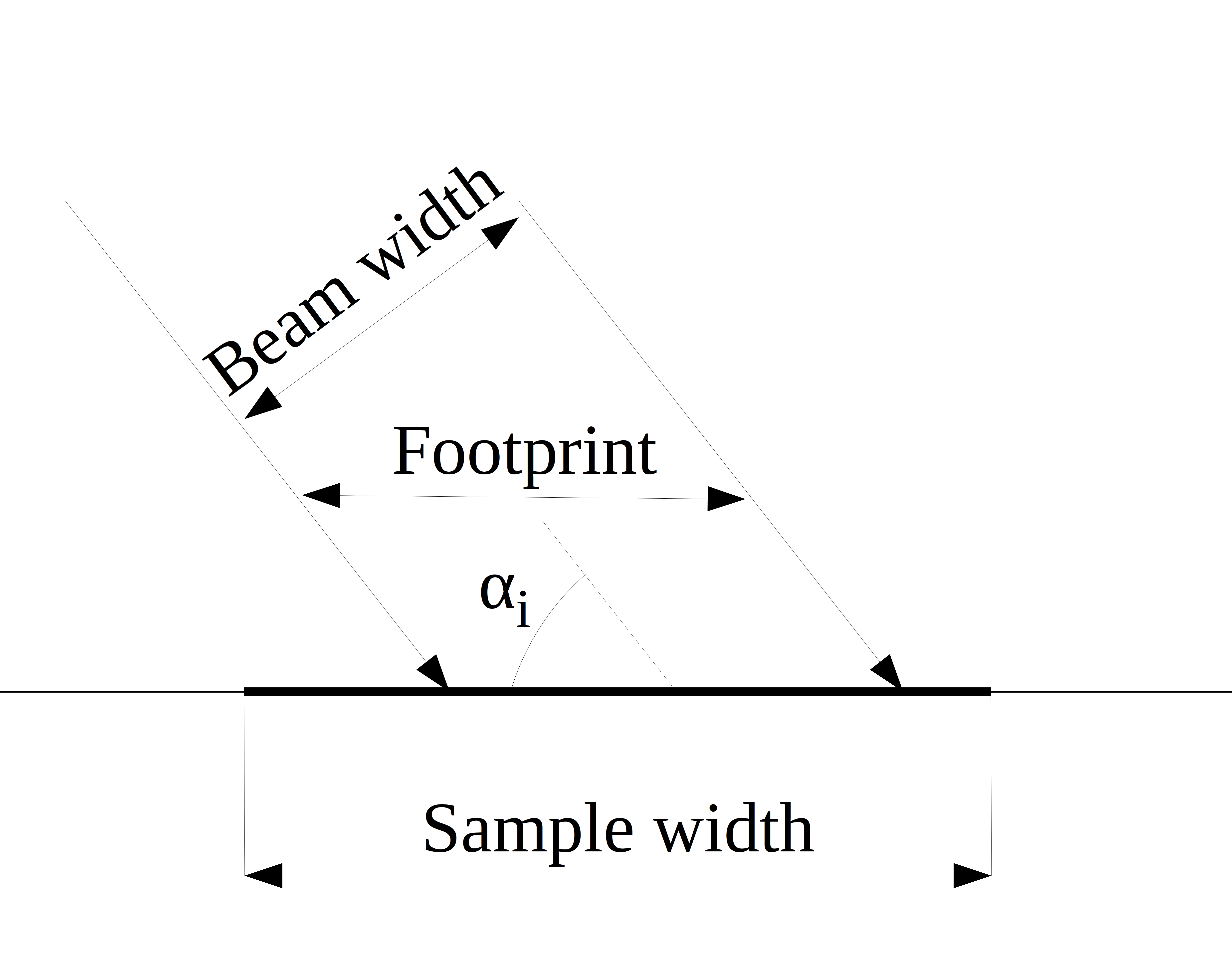
Footprint scene
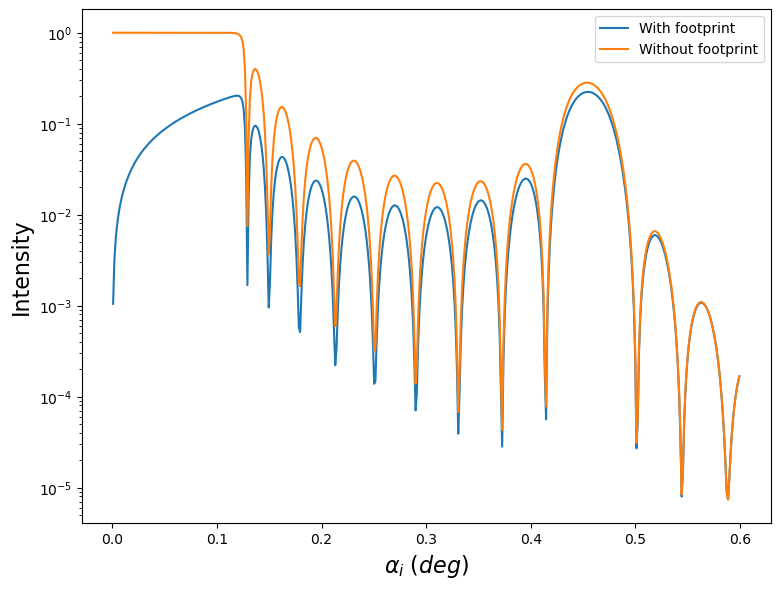
Intensity image
When taking into account footprint correction, there are two possible options for the
beam shape in BornAgain:
The footprint correction for square beam is defined by
FootprintSquare command, which has the signature
<footprint_object> = FootprintSquare(beam_to_sample_width_ratio)
Here <footprint_object> is an object later passed to the simulation, while beam_to_sample_width_ratio
defines the ratio between the widths of beam and sample.
In the case of the Gaussian beam the footprint object is created with
<footprint_object> = FootprintGauss(beam_to_sample_width_ratio)
The command signature is exactly the same as in the case with the square beam,
but the beam width required for beam_to_sample_width_ratio
is now defined as the beam diameter associated with the intensity level equal to $I_0 \cdot e^{-\frac{1}{2}}$,
where $I_0$ is the on-axis (maximal) intensity.
In this example a square beam is considered, with beam_to_sample_width_ratio being equal to $0.01$.
The incident angle range was made rather small in this example
(from $0.0$ to $0.6$ degrees) in order to emphasize
the footprint impact at small incident angles.
In other respects this example exactly matches the
reflectometry simulation tutorial.
|
|