  1
  2
  3
  4
  5
  6
  7
  8
  9
 10
 11
 12
 13
 14
 15
 16
 17
 18
 19
 20
 21
 22
 23
 24
 25
 26
 27
 28
 29
 30
 31
 32
 33
 34
 35
 36
 37
 38
 39
 40
 41
 42
 43
 44
 45
 46
 47
 48
 49
 50
 51
 52
 53
 54
 55
 56
 57
 58
 59
 60
 61
 62
 63
 64
 65
 66
 67
 68
 69
 70
 71
 72
 73
 74
 75
 76
 77
 78
 79
 80
 81
 82
 83
 84
 85
 86
 87
 88
 89
 90
 91
 92
 93
 94
 95
 96
 97
 98
 99
100
101
102
103
104
105
106
107
108
109
110
111
112
113
114
115
116
117
118
119
120
121
122
123
|
#!/usr/bin/env python3
"""
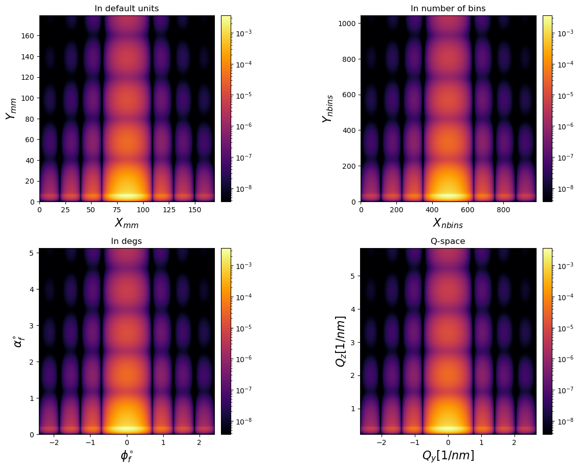
In this example we demonstrate how to plot simulation results with
axes in different units (nbins, mm, degs and QyQz).
"""
import bornagain as ba
from bornagain import angstrom, deg, nm, nm2, kvector_t
import ba_plot
from matplotlib import pyplot as plt
from matplotlib import rcParams
def get_sample():
"""
Returns a sample with uncorrelated cylinders on a substrate.
"""
# Define materials
material_Particle = ba.HomogeneousMaterial("Particle", 0.0006, 2e-08)
material_Substrate = ba.HomogeneousMaterial("Substrate", 6e-06, 2e-08)
material_Vacuum = ba.HomogeneousMaterial("Vacuum", 0, 0)
# Define form factors
ff = ba.FormFactorCylinder(5*nm, 5*nm)
# Define particles
particle = ba.Particle(material_Particle, ff)
# Define particle layouts
layout = ba.ParticleLayout()
layout.addParticle(particle)
layout.setTotalParticleSurfaceDensity(0.01)
# Define layers
layer_1 = ba.Layer(material_Vacuum)
layer_1.addLayout(layout)
layer_2 = ba.Layer(material_Substrate)
# Define sample
sample = ba.MultiLayer()
sample.addLayer(layer_1)
sample.addLayer(layer_2)
return sample
def get_simulation(sample):
beam = ba.Beam(1, 1*angstrom, ba.Direction(0.2*deg, 0))
# PILATUS detector
detector_distance = 2000.0 # in mm
pilatus_pixel_size = 0.172 # in mm
pilatus_npx, pilatus_npy = 981, 1043 # number of pixels
width = pilatus_npx*pilatus_pixel_size
height = pilatus_npy*pilatus_pixel_size
detector = ba.RectangularDetector(pilatus_npx, width, pilatus_npy,
height)
detector.setPerpendicularToSampleX(detector_distance, width/2., 0)
simulation = ba.GISASSimulation(beam, sample, detector)
return simulation
def run_simulation():
simulation = get_simulation(get_sample())
simulation.runSimulation()
return simulation.result()
def plot(result):
"""
Plots simulation results for different detectors.
"""
# set plotting parameters
rcParams['image.cmap'] = 'jet'
rcParams['image.aspect'] = 'auto'
fig = plt.figure(figsize=(12.80, 10.24))
plt.subplot(2, 2, 1)
# default units for rectangular detector are millimeters
ba_plot.plot_colormap(result,
title="In default units",
xlabel=r'$X_{mm}$',
ylabel=r'$Y_{mm}$',
zlabel=None)
plt.subplot(2, 2, 2)
ba_plot.plot_colormap(result,
units=ba.Axes.NBINS,
title="In number of bins",
xlabel=r'$X_{nbins}$',
ylabel=r'$Y_{nbins}$',
zlabel=None)
plt.subplot(2, 2, 3)
ba_plot.plot_colormap(result,
units=ba.Axes.DEGREES,
title="In degs",
xlabel=r'$\phi_f ^{\circ}$',
ylabel=r'$\alpha_f ^{\circ}$',
zlabel=None)
plt.subplot(2, 2, 4)
ba_plot.plot_colormap(result,
units=ba.Axes.QSPACE,
title="Q-space",
xlabel=r'$Q_{y} [1/nm]$',
ylabel=r'$Q_{z} [1/nm]$',
zlabel=None)
plt.subplots_adjust(left=0.07,
right=0.97,
top=0.9,
bottom=0.1,
hspace=0.25)
plt.show()
if __name__ == '__main__':
result = run_simulation()
plot(result)
|