Bayesian sampling

Bayesian sampling of reflectometry models is a common tool in the analysis of specular reflectometry data. The Python programming language has a powerful infrastructure for this modelling, including packages such as PyMC3 and PyStan. Here, we will show how the emcee Python may be used to enable Bayesian sampling in BornAgain and the differential evoulation optimisation algorithm from the scipy.

Example script

To generate these images of the probability distributions of the parameters and the maximum likelihood reflectometry profile

run this script

  1
  2
  3
  4
  5
  6
  7
  8
  9
 10
 11
 12
 13
 14
 15
 16
 17
 18
 19
 20
 21
 22
 23
 24
 25
 26
 27
 28
 29
 30
 31
 32
 33
 34
 35
 36
 37
 38
 39
 40
 41
 42
 43
 44
 45
 46
 47
 48
 49
 50
 51
 52
 53
 54
 55
 56
 57
 58
 59
 60
 61
 62
 63
 64
 65
 66
 67
 68
 69
 70
 71
 72
 73
 74
 75
 76
 77
 78
 79
 80
 81
 82
 83
 84
 85
 86
 87
 88
 89
 90
 91
 92
 93
 94
 95
 96
 97
 98
 99
100
101
102
103
104
105
106
107
108
109
110
111
112
113
114
115
#!/usr/bin/env python3
"""
An example of using the Bayesian sampling library emcee with BornAgain.

Author: Andrew McCluskey (andrew.mccluskey@ess.eu)
"""

import bornagain as ba, corner, emcee, numpy as np, os, scipy
import matplotlib.pyplot as plt
from bornagain import nm

np.random.seed(1)

datadir = os.getenv('BA_DATA_DIR', '')


def get_sample(ni_thickness, ti_thickness):
    # pure real scattering-length densities (in angstrom^-2)
    si_sld_real = 2.0704e-06  # Si (substrate)
    ni_sld_real = 9.4245e-06  # Ni
    ti_sld_real = -1.9493e-06  # Ti

    # materials
    vacuum = ba.MaterialBySLD()
    material_ni = ba.MaterialBySLD("Ni", ni_sld_real, 0)
    material_ti = ba.MaterialBySLD("Ti", ti_sld_real, 0)
    material_substrate = ba.MaterialBySLD("SiSubstrate", si_sld_real, 0)

    # multilayer
    vacuum_layer = ba.Layer(vacuum)
    ni_layer = ba.Layer(material_ni, ni_thickness)
    ti_layer = ba.Layer(material_ti, ti_thickness)
    substrate_layer = ba.Layer(material_substrate)
    sample = ba.MultiLayer()
    sample.addLayer(vacuum_layer)
    for _ in range(10):
        sample.addLayer(ti_layer)
        sample.addLayer(ni_layer)
    sample.addLayer(substrate_layer)
    return sample


def get_simulation(sample, points):
    scan = ba.AlphaScan(ba.ListScan("alpha_i (rad)", points))
    scan.setWavelength(0.154 * nm);
    return ba.SpecularSimulation(scan, sample)


def run_simulation(points, ni_thickness, ti_thickness):
    sample = get_sample(ni_thickness, ti_thickness)
    simulation = get_simulation(sample, points)

    result = simulation.simulate()
    return result.npArray()


if __name__ == '__main__':
    filepath = os.path.join(datadir, "specular/genx_alternating_layers.dat.gz")
    flags = ba.ImportSettings1D("2alpha (deg)", "#", "", 1, 2)
    data = ba.readData1D(filepath, ba.csv1D, flags)

    q = data.npXcenters()
    y = data.npArray()
    dy = y * 0.1 # arbitrary uncertainties

    def log_likelihood(P):
        """
        Calculates the log-likelihood for the normal uncertainties
        :tuple sim_var: the variable parameters
        :array x: the abscissa data (q-values)
        :array y: the ordinate data (R-values)
        :array yerr: the ordinate uncertainty (dR-values)
        :return: log-likelihood
        """
        y_sim = run_simulation(q, *P)
        sigma2 = dy**2 + y_sim**2
        return -0.5*np.sum((y - y_sim)**2/sigma2 + np.log(sigma2))

    # Use differential evolution to find the maximum likelihood estimate
    objective_function = lambda *args: -log_likelihood(*args) # just change sign
    initial = np.array([9.0, 1.0]) + 0.1*np.random.randn(2)
    solution = scipy.optimize.differential_evolution(
        objective_function,
        bounds=((5.0, 9.0), (1.0, 10.0)))

    ni_thickness_ml, ti_thickness_ml = solution.x
    print('MLE Ni Thickness', ni_thickness_ml, 'nm')
    print('MLE Ti Thickness', ti_thickness_ml, 'nm')

    # Perform the likelihood sampling
    nwalkers = 32
    ndim = 2
    pos = solution.x + 1e-4*np.random.randn(nwalkers, ndim)
    sampler = emcee.EnsembleSampler(nwalkers,
                                    ndim,
                                    log_likelihood)
    sampler.run_mcmc(pos, 1000, progress=True)

    # Plot and show corner plot of samples
    flat_samples = sampler.get_chain(flat=True)
    corner.corner(flat_samples,
                  labels=['Ni-thickness/nm', 'Ti-thickness/nm'])
    plt.show()

    # Plot and show MLE and data of reflectivity
    plt.errorbar(q, y, dy, marker='.', ls='')
    plt.plot(
        q,
        run_simulation(q, *flat_samples.mean(axis=0)),
        '-')
    plt.xlabel('$\\alpha$/rad')
    plt.ylabel('$R$')
    plt.yscale('log')
    plt.show()
auto/Examples/bayesian/likelihood_sampling.py

Explanation

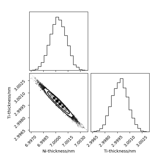
The system under investigation in the above example is a Ni-Ti multilayer material at the interface between an Si substrate and a vacuum. There are two parameters of interest, the thicknesses of the Ni and Ti layers. We know the scattering length densities for each, and that in total there are 10 repetitions of the Ni-Ti sandwich. This sample is created in the get_sample function.

Having built the sample, it is necessary to obtain the real experimental data. For the above code to work locally, the data file genx_alternating_layers.dat.gz is required and the Python script (in particular the get_real_data function) should be adapted appropriately. This function defined an uncertainty in the reflectivity of 10 %.

The simulation is then defined in the get_simulation function, which is passed a series of angles, however, this may be modified to perform a Q-scan as necessary. The final function that is necessary is the simulation of specular reflectometry is the run_simulation function. This will take the angle-value to be simulated and thickness for the Ni and Ti layers and then return the result of the simulation as a numpy.array.

We will use the emcee package to sampling the likelihood of the data (we are follow their data fitting example). Therefore, it is necessary to define a likelihood (the log_likelihood function) objective. Then, within the main body of the scirpt we firstly find the maximum likelihood solution using a differential evolution algorithm from the scipy.optimize library. This should print that then thicknesses are around 7 nm and 3 nm for the Ni and Ti respectively.

We can use the emcee.EnsembleSampler to probe the uncertainties in the parameters and there correlation. This will perform the sampling for some time (on my machine it took about 2.5 minutes to sample 1000 steps with 32 walkers). Having collected the samples, we can then unpack them and using the corner package visualise them. This will give the first image shown above.

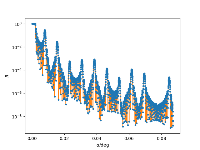
Finally, we can plot the maximum likelihood estimate for the model along with the experimental data. This is the second image above.

Note that the flat_samples object describes the distributions shown in the corner plot. Therefore we can find values of interest, such as the standard deviation or confident intervals.