The basic features of the interface are explained below.
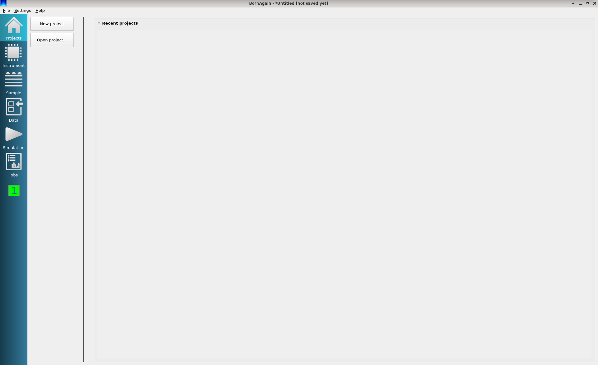
When you start BornAgain GUI, you will be presented with the Projects View, where you can
You can use the view selector located on the left vertical panel (1) to change to one of the following views.

|
Switch to Projects View |

|
Define the instrument geometry: beam and detector parameters |

|
Build the sample |

|
Import experimental data to fit |

|
Run a simulation |

|
Switch to see job results, tune parameters in real time, fit the data |
The Instrument View is used to create new scattering instruments and adjust their settings. The view consists of the instrument selector located on the left (1) and the instrument settings window located on the right (2).
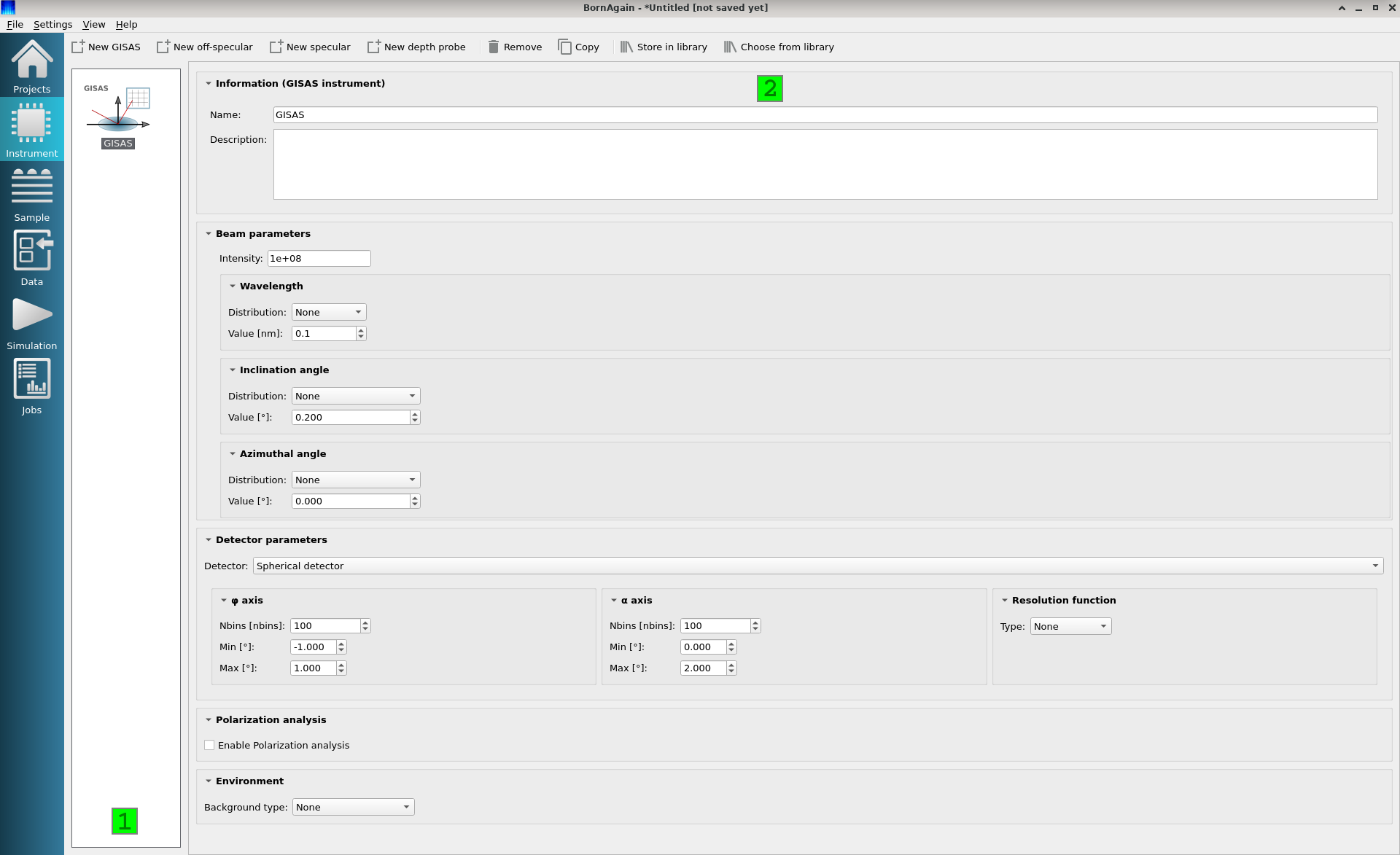
On the instrument settings window (2) you can modify the settings of the currently selected instrument:
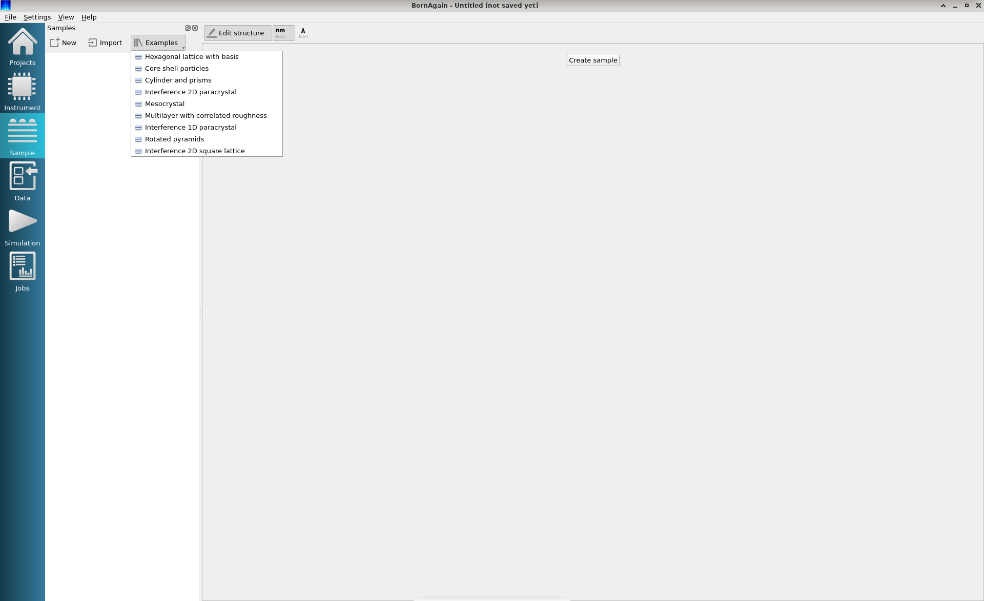
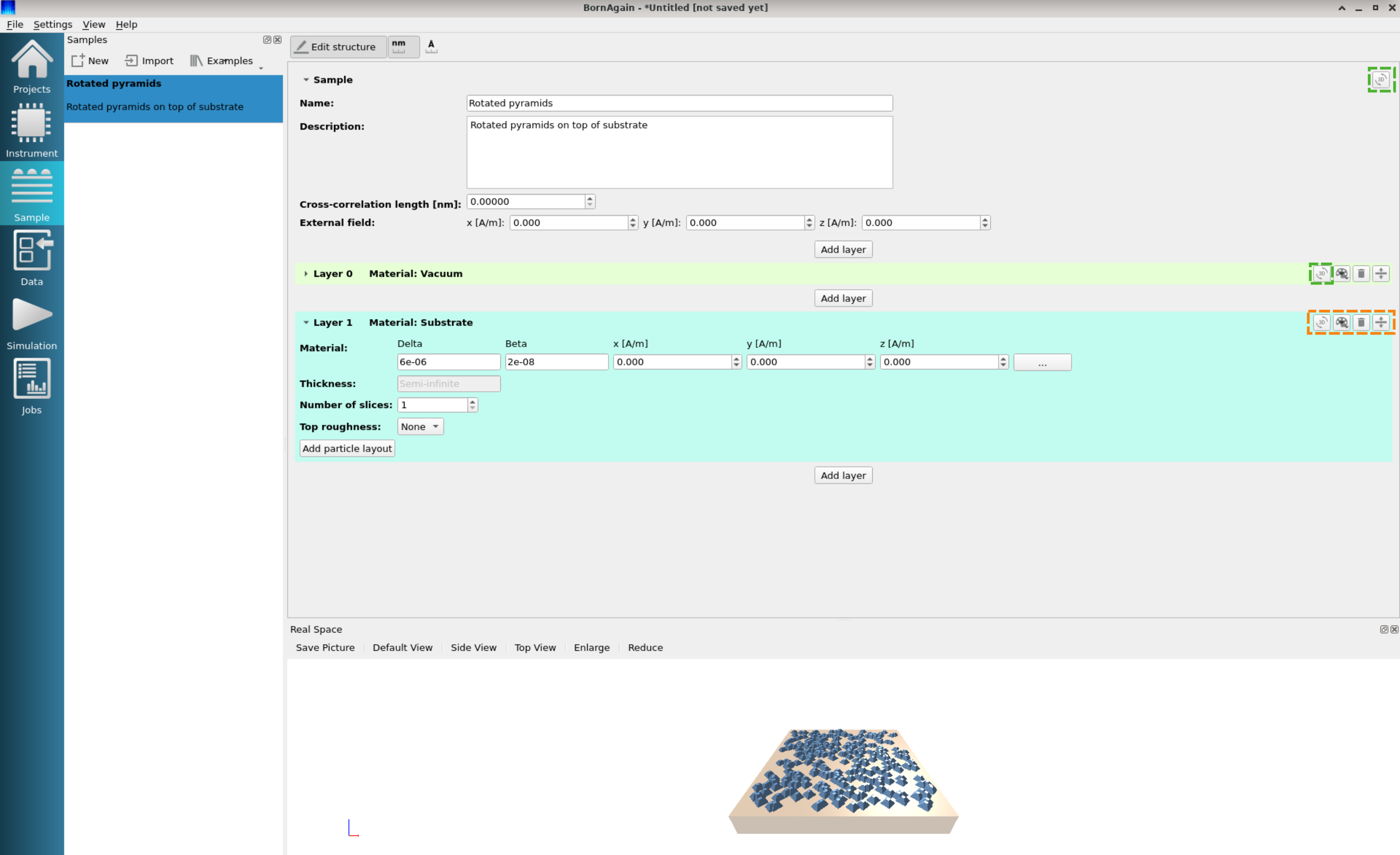
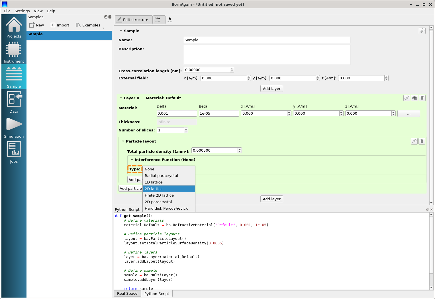
The Sample View allows you to design the sample via a graphical interface. For simplicity, one can start with a predefined sample from the Examples menu.
Here, the “Rotated pyramids” predefined sample is selected. The model consists of two layers, “Vacuum” and “Substrate”, which are distinguished by colors. A manipulatable 3d graphical representation of the sample is displayed in the Real Space pane.
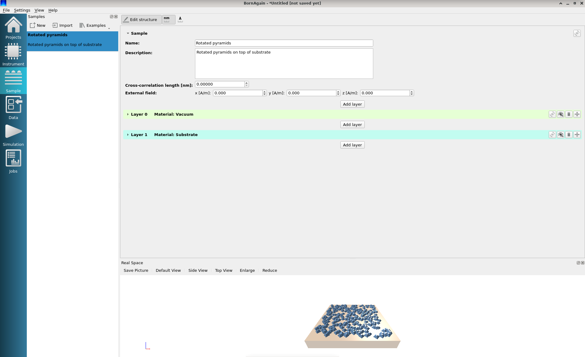
The defining parameters of each layer can be shown and modified by expanding the layer.

The layers can be moved up or down, or removed from the sample using the set of buttons on the right (denoted by an orange rectangle).
Note that vertical order of layers represent the same order in the real space
(for instance, in the image below, Layer 0 is on top of Layer 1).
The color of the layer can also be changed with these buttons.
The 3d representation of each layer can be shown separately by clicking the 3D button for each layer (denoted by green rectangles). To display the 3d representation of the full sample, press the 3d button of the Sample.
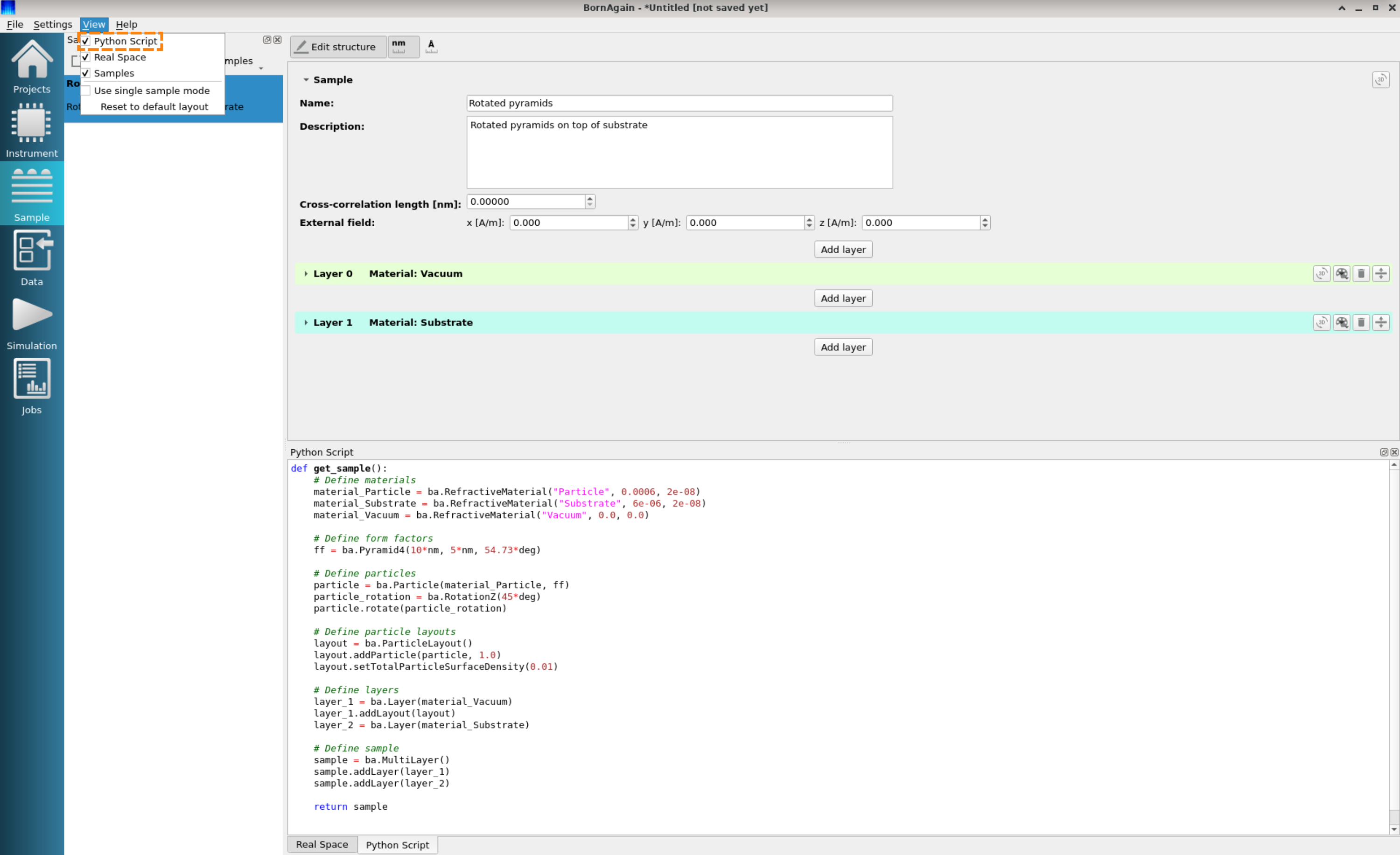
The Python script corresponding to the sample can be displayed by checking View→Python Script.
To construct a new sample from scratch, one should use the “New” button and then add a layer by clicking the “Add layer” button.
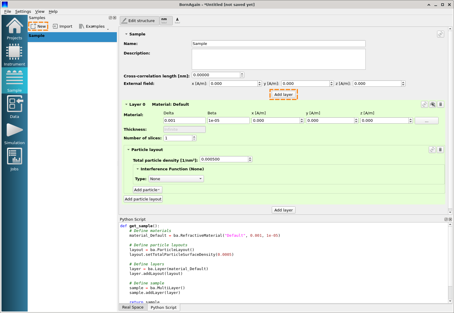
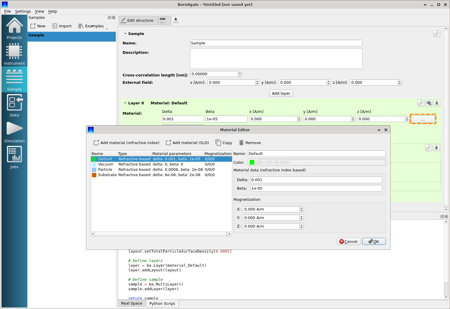
The material of the layer can be changed via the material editor. Note that the default material is vacuum.
The interference function (particle layout) can be selected via the Type drop-down menu.
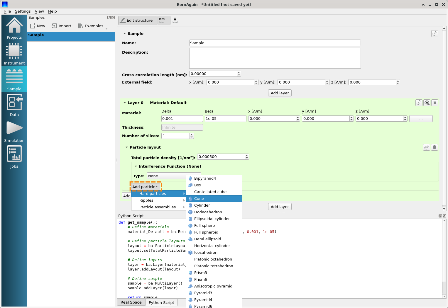
The type of the particles can be selected via the “Add particle” menu.
In the same way, the user can create an arbitrary number of samples, each with an arbitrary number of layers. If this is the case, during the configuration of the simulation the user will have to choose which sample for the simulation. The sample is considered as valid for the simulation, if it contains at least one layer.
The Simulation View contains the following parts
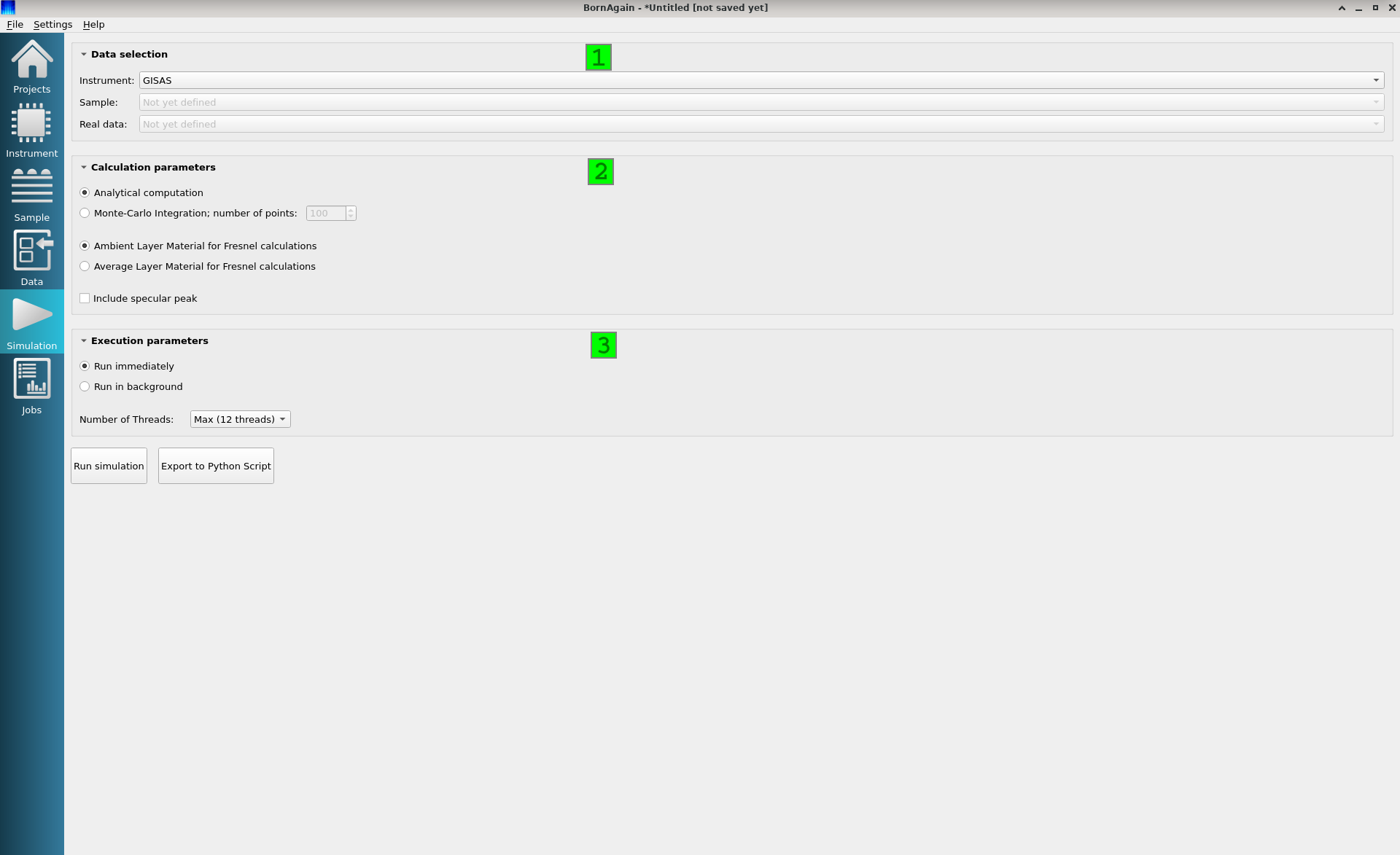
The names of the defined instruments and samples are displayed in the Data Selection box (1). There, the user can select a combination for running a simulation.
Clicking on the “Run Simulation” button immediately starts the simulation. When completed, the current view is automatically switched to the Jobs View showing the simulation results. This behaviour can be modified by changing to “Run in Background” in (3).
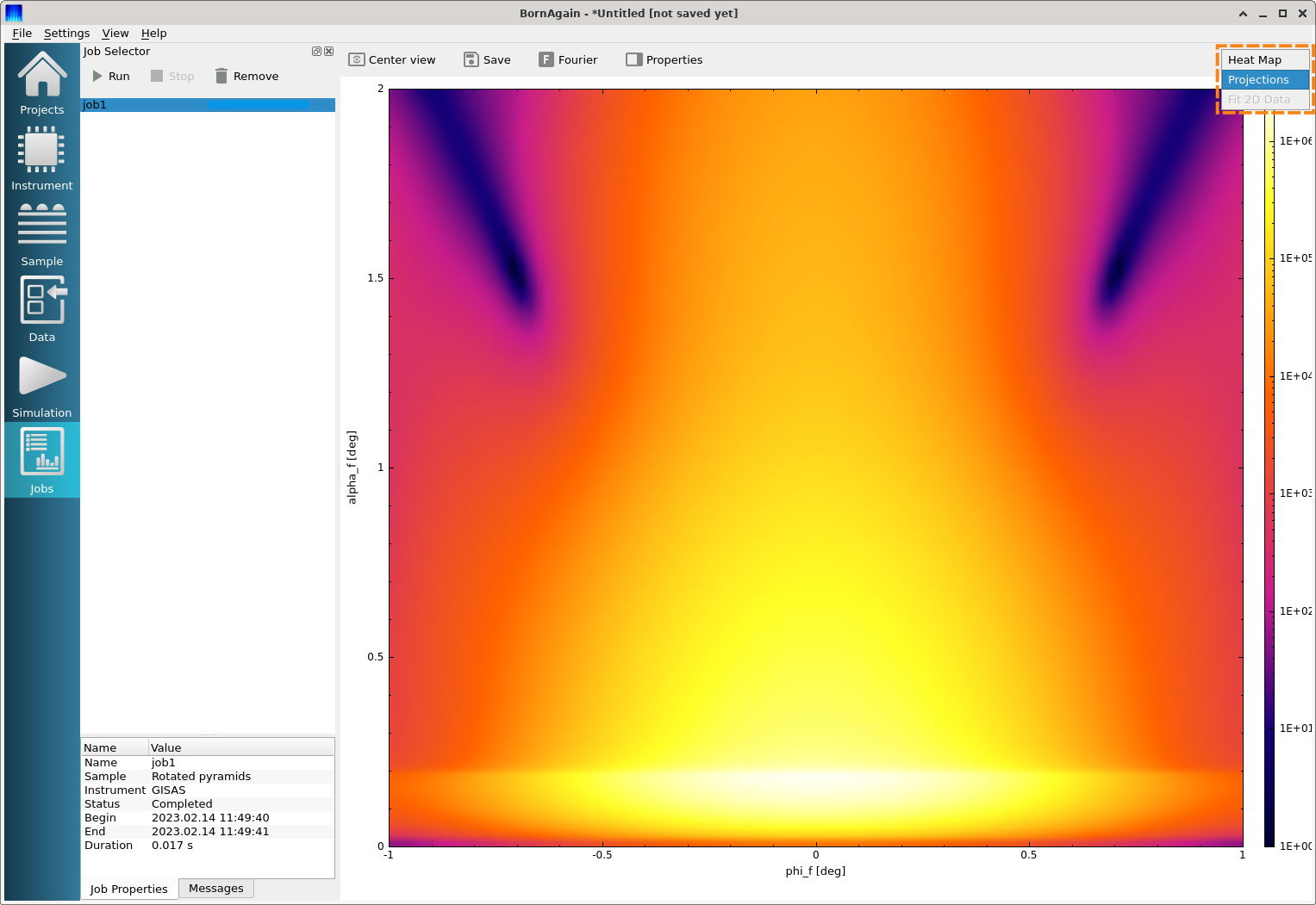
The Jobs View displays the results of the simulation. It has two different presentations called
Job View Activity is shown by default.
The layout of the Job View Activity consists of five elements
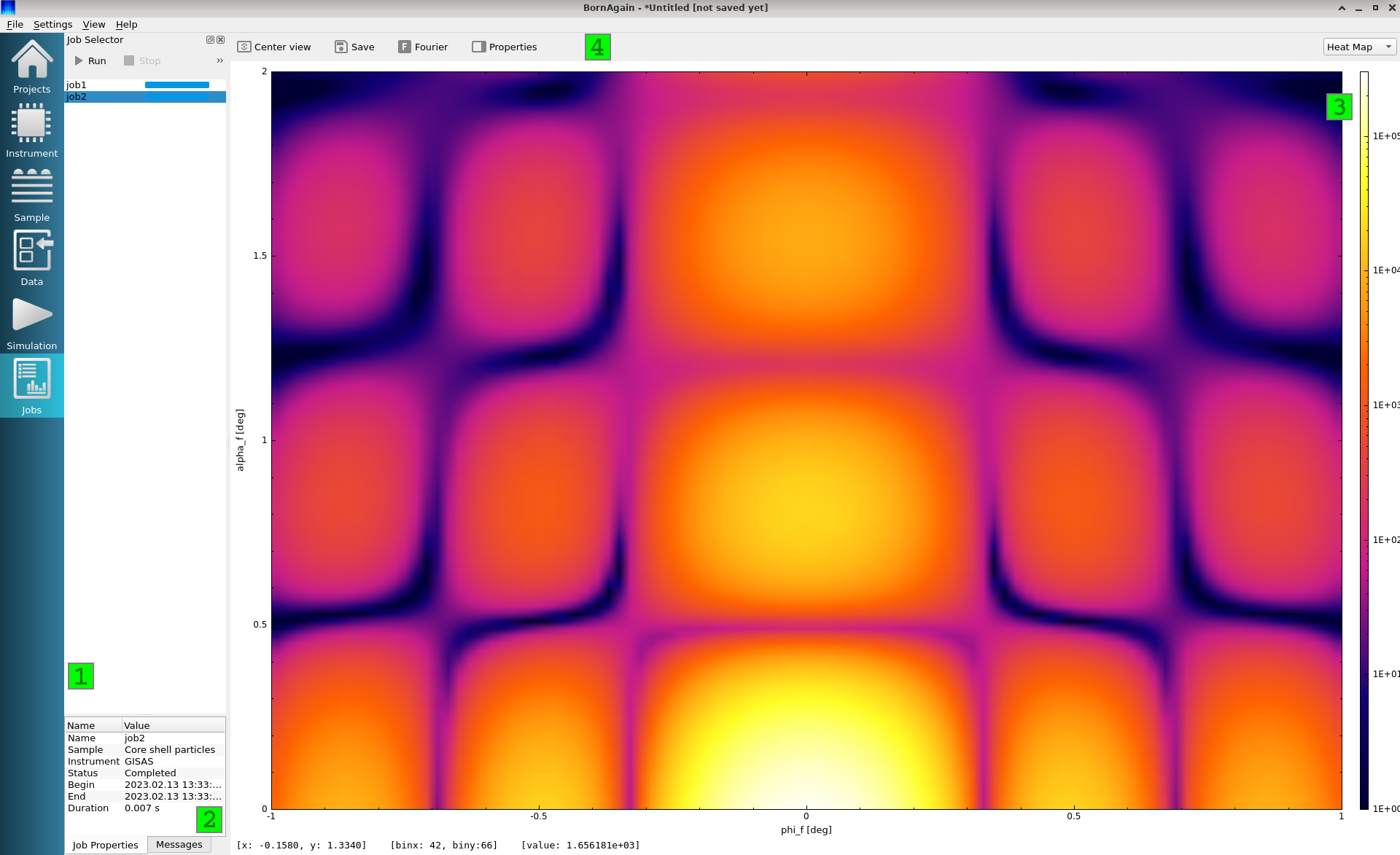
The two completed jobs can be seen in the job selector widget (1), with
job2currently selected and displayed.
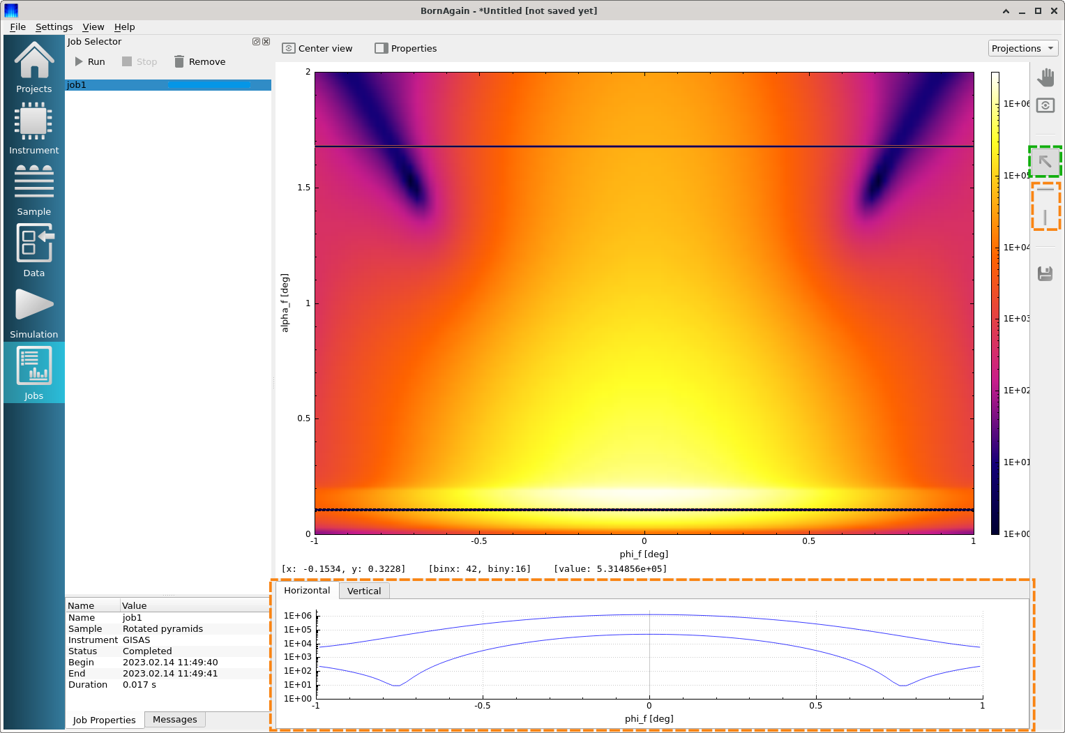
The intensity image in widget (3) offers several ways of interaction:
The Projections panel is accessible from the drop-down menu on the upper right-hand side of the Jobs View.
Horizontal or vertical projections can be added to the image via the buttons on the toolbar on the right-hand side. The projection plots will be displayed in the pane below the image; note the orange rectangles.
The projections can be selected via the arrow icon (denoted by a green rectangle). The selected projection can be moved using arrow keys or the mouse.
It can be deleted by pressing the Delete key.
The “Real Time Activity” panel can be switched on by View → Real Time Activity.

Switching to “Real Time Activity” will display a parameter tree (denoted by an orange rectangle) which represents the set of all parameters that have been used during the construction of the scattering instrument and the sample. Each displayed parameter value can be adjusted using a slider. The simulation will run in the background and the intensity image will be constantly updated reflecting the influence of the given parameter on the simulation results.
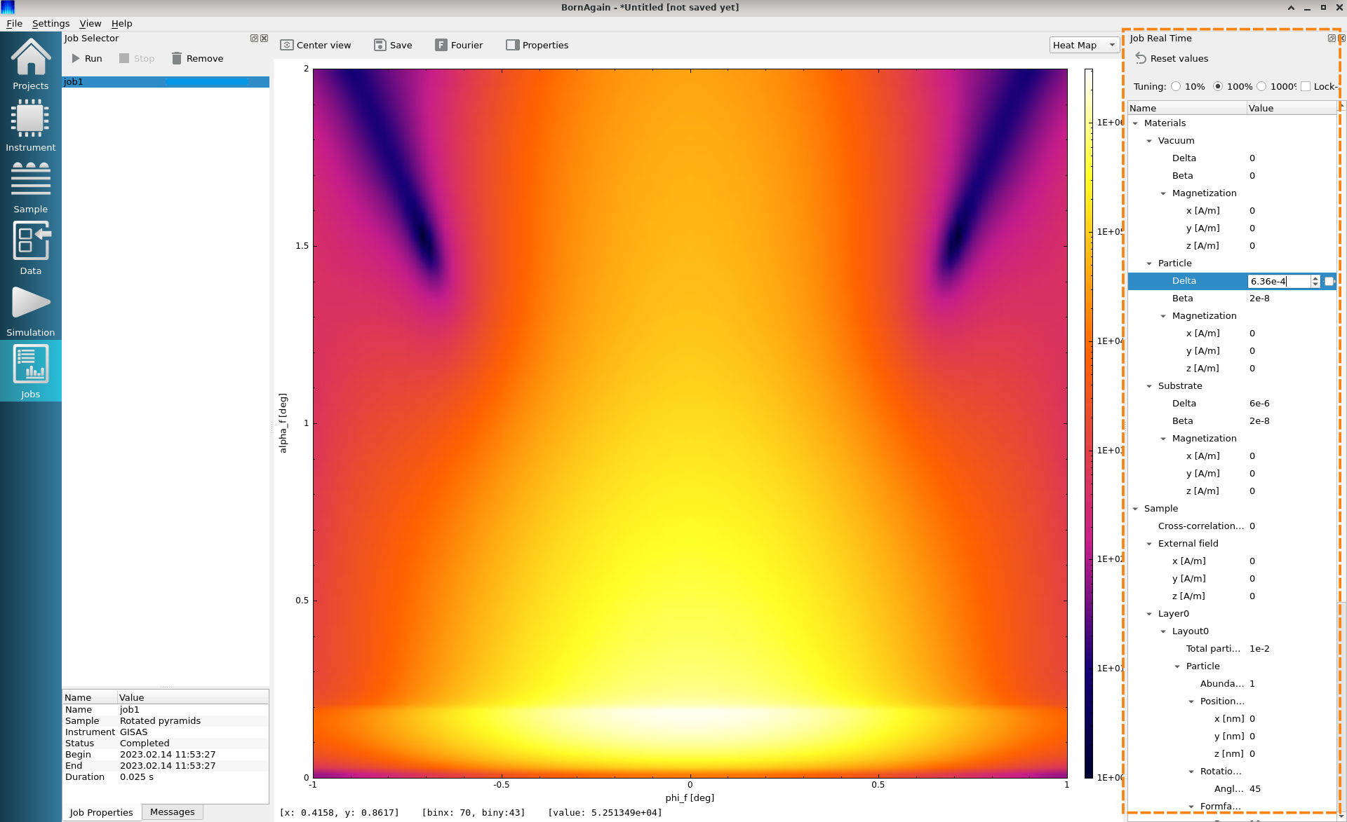
Note
The Real Time View works smoothly only for simple geometries, when the simulation requires fractions of a second to run. For more complex geometries, demanding more CPU power, the user will see a progress bar and any movements of the slider will not have a direct influence on the produced image (Intensity Data widget). In this case the user may try to speed up the simulation by decreasing the number of detector channels in the Instrument View and submitting a new job by running the simulation from the Simulation View.
Important
The jobs in the Jobs View are completely isolated from the rest of the program. Any adjustments of the sample parameters in the Sample View or the instrument parameters in the Instrument View won’t have any influence on the jobs already completed or still running in the Jobs View. Similarly, in “Real Time Activity” mode, any parameter adjustments made in the parameter tree will not be propagated back into the Sample or Instrument Views.