Reflectometry: Fit Pt layer

In this example, we want to demonstrate how to fit experimental reflectivity data that was obtained by a time-of-flight experiment with unpolarized neutrons. Experimental data is available for a sample of a roughly 50 nm thick platinum layer on top of a silicon substrate that is published in this repository.

The mesaurements were made by Timothy Charlton, Haile Ambaye and Michael Fitzsimmons (ORNL) on a sample provided by Eric Fullerton (UCSD).

Fit model

We describe the above experiment by a three-layer model, where as usual the top layer is the vacuum and the substrate layer is the silicon substrate. On top of the silicon substrate, we place the platinum layer. The materials of both layers are described by their SLD, where we use literature values for both silicon as well as platinum and keep them constant throughout the fitting procedure.

The main parameters of the sample are stored in dictionary, where they are defined by a unique name and the following six parameters are utilized:

  • Beam intensity: intensity

    We explicitly fit the beam intensity, in order to compensate for possible experimental errors and to circumvent problems with the rather large variance in the reflectivity data at low $Q$-values.

  • Roughness on top of the Pt layer: r_pt/nm

  • Roughness on top of the Si substrate: r_si/nm

  • Thickness of the Pt layer: t_pt/nm

  • The relative $Q$-resolution: q_res/q (c.f.)

  • A $Q$-offset: q_offset

This global offset is introduced to account for uncertainties in the angle at which the measurement is performed.

Due to saturation of the detector it is possible that the intensity at low $Q$-values (i.e. at high count rates) is underestimated. Furthermore, there is a rather large variance in the data that also leads to a rather bad fit in this region. Therefore, we neglect the data in the low $Q$-region by choosing a cutoff at $Q_{\text{min}} = $ 0.18. This value is selected by hand after performing several fits and visually selecting a good result.

$Q$-offset

Currently, BornAgain does not have an API support for an offset of the $Q$-axis. Therefore, we need to shift the $Q$-axis before performing a simulation

q_axis = q_axis + parameters["q_offset"]

This shift then needs to be counter-transformed when returning the results in the qr(result) function

q = numpy.array(result.result().axis(ba.Axes.QSPACE)) - q_offset
Initial parameters

In order to successfully fit this example, we chose some sane starting values and the example code that is fully given below, can be run with the following command:

python3 Pt_layer_fit.py fit

This performs a simulation with the initial parameters and yields the following result:

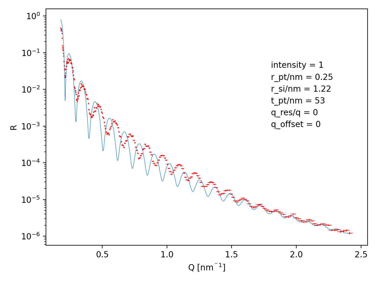
Reflectivity with the initial parameters before fitting

Immediately afterwards the fit is performed.

Fit result

In order to run the fitting procedure, the following command can be issued:

python3 Pt_layer_fit.py fit

We need to allow a few seconds computational time and BornAgain should compute the following result

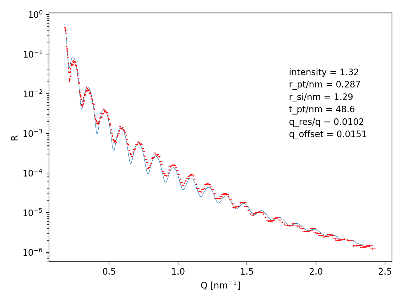
Reflectivity with the parameters obtained from our fit

If the fit keyword is omitted from the command line

python3 Pt_layer_fit.py

a simulation is performed with our fit results and one should obtain the result shown above.

  1
  2
  3
  4
  5
  6
  7
  8
  9
 10
 11
 12
 13
 14
 15
 16
 17
 18
 19
 20
 21
 22
 23
 24
 25
 26
 27
 28
 29
 30
 31
 32
 33
 34
 35
 36
 37
 38
 39
 40
 41
 42
 43
 44
 45
 46
 47
 48
 49
 50
 51
 52
 53
 54
 55
 56
 57
 58
 59
 60
 61
 62
 63
 64
 65
 66
 67
 68
 69
 70
 71
 72
 73
 74
 75
 76
 77
 78
 79
 80
 81
 82
 83
 84
 85
 86
 87
 88
 89
 90
 91
 92
 93
 94
 95
 96
 97
 98
 99
100
101
102
103
104
105
106
107
108
109
110
111
112
113
114
115
116
117
118
119
120
121
122
123
124
125
126
127
128
129
130
131
132
133
134
135
136
137
138
139
140
141
142
143
144
145
146
147
148
149
150
151
152
153
154
155
156
157
158
159
160
161
162
163
#!/usr/bin/env python3
"""
Fit example with data by M. Fitzsimmons et al,
https://doi.org/10.5281/zenodo.4072376.
Sample is a ~50 nm Pt film on a Si substrate.
Single event data from Spallation Neutron Source
Beamline-4A (MagRef) with 60 Hz pulses and a wavelength
band of roughly 4-7 Å in 100 steps of 2theta.
"""

import bornagain as ba, numpy as np, os, matplotlib.pyplot as plt
from bornagain import angstrom

datadir = os.getenv('BA_DATA_DIR', '')

####################################################################
#  Sample and simulation model
####################################################################

# Use fixed values for the SLD of the substrate and Pt layer
sldPt = (6.3568e-06, 1.8967e-09)
sldSi = (2.0728e-06, 2.3747e-11)

def get_sample(P):

    vacuum = ba.MaterialBySLD("Vacuum", 0, 0)
    material_layer = ba.MaterialBySLD("Pt", *sldPt)
    material_substrate = ba.MaterialBySLD("Si", *sldSi)

    ambient_layer = ba.Layer(vacuum)
    layer = ba.Layer(material_layer, P["t_pt/nm"])
    substrate_layer = ba.Layer(material_substrate)

    r_si = ba.LayerRoughness(P["r_si/nm"])
    r_pt = ba.LayerRoughness(P["r_pt/nm"])

    sample = ba.MultiLayer()
    sample.addLayer(ambient_layer)
    sample.addLayerWithTopRoughness(layer, r_pt)

    sample.addLayerWithTopRoughness(substrate_layer, r_si)

    return sample


def get_simulation(q_axis, P):
    sample = get_sample(P)

    scan = ba.QzScan(q_axis)
    scan.setIntensity(P["intensity"])
    scan.setOffset(P["q_offset"])

    distr = ba.DistributionGaussian(0., 1., 25, 4.)
    scan.setAbsoluteQResolution(distr, P["q_res/q"])

    simulation = ba.SpecularSimulation(scan, sample)

    return simulation

####################################################################
#  Plotting
####################################################################

def plot(q, r, data, P):
    fig = plt.figure()
    ax = fig.add_subplot(111)

    ax.errorbar(data.npXcenters(),
                data.npArray(),
                # xerr=data.xxx, TODO restore
                yerr=data.npErrors(),
                label="R",
                fmt='.',
                markersize=1.,
                linewidth=0.6,
                color='r')

    ax.plot(q, r, label="Simulation", color='C0', linewidth=0.5)

    ax.set_yscale('log')

    ax.set_xlabel("$q\;$(nm$^{-1}$)")
    ax.set_ylabel("$R$")

    y = 0.5
    if P is not None:
        for n, v in P.items():
            plt.text(0.7, y, f"{n} = {v:.3g}", transform=ax.transAxes)
            y += 0.05

    plt.tight_layout()
    

####################################################################
#  Main
####################################################################

if __name__ == '__main__':

    # Parameters and bounds:

    fixedPnB = {
        # to keep some parameters fixed, move lines here from startPnB
    }

    startPnB = {
        "intensity": (1., 0.8, 1.2),
        "q_offset": (0.01, -0.02, 0.02),
        "q_res/q": (0.01, 0, 0.02),
        "t_pt/nm": (50, 45, 55),
        "r_si/nm": (1.22, 0, 5),
        "r_pt/nm": (0.25, 0, 5),
    }

    fixedP = {d: v[0] for d, v in fixedPnB.items()}
    initialP = {d: v[0] for d, v in startPnB.items()}

    # Set q axis, load data:

    qmin = 0.18
    qmax = 2.4
    qzs = np.linspace(qmin, qmax, 1500)

    fpath = os.path.join(datadir, "specular/RvsQ_36563_36662.dat.gz")
    flags = ba.ImportSettings1D("q (1/angstrom)", "#", "", 1, 2, 3, 4)
    data = ba.readData1D(fpath, ba.csv1D, flags)

    # Initial plot

    r = get_simulation(qzs, initialP | fixedP).simulate().npArray()
    plot(qzs, r, data, initialP)

    # Restrict data to given q range

    data = data.crop(qmin, qmax)

    # Fit:

    fit_objective = ba.FitObjective()
    fit_objective.setObjectiveMetric("chi2")
    fit_objective.initPrint(10)
    fit_objective.addFitPair(
        lambda P: get_simulation(data.npXcenters(), P | fixedP), data, 1)

    P = ba.Parameters()
    for name, p in startPnB.items():
        P.add(name, p[0], min=p[1], max=p[2])

    minimizer = ba.Minimizer()
    result = minimizer.minimize(fit_objective.evaluate, P)
    fit_objective.finalize(result)

    finalP = {r.name(): r.value for r in result.parameters()}

    # Print and plot fit outcome:

    print("Fit Result:")
    print(finalP)

    r = get_simulation(qzs, finalP | fixedP).simulate().npArray()
    plot(qzs, r, data, finalP)

    plt.show()
auto/Examples/fit/specular/Pt_layer_fit.py

Data to be fitted: RvsQ_36563_36662.txt.gz