The interference function of a two-dimensional lattice is used to model the scattering from particles positioned at some regular intervals.
The generated layout, the lattice, is characterised by two basis vectors $a$ and $b$ (in real space) and the angle between these two vectors. The finite size effects and/or divergence of the lattice from an ideal crystal are modelled with the help of two-dimensional decay functions.
See BornAgain user manual (Chapter 3.4.2, Two Dimensional Lattice) for details about the theory.
The interference function is created using its constructor
Interference2DLattice(length_1, length_2, alpha, xi=0.0)
"""
length1, length2 : lengths of the basis vectors, in nanometers
alpha            : angle between the basis vectors, in radians
xi               : rotation of the lattice with respect to the x-axis, in radians
"""
length1 and length2 are the lengths of basis vectors $a$ and $b$ expressed in nanometers (see plot below). alpha ($\alpha$) is the angle between the two basis vectors $a$, $b$ (in radians). xi ($\xi$) is the angle defining the lattice orientation. It is taken as the angle between the first basis vector $a$ and the x-axis of the Cartesian coordinate system. It is expressed in radians and set to 0 by default.
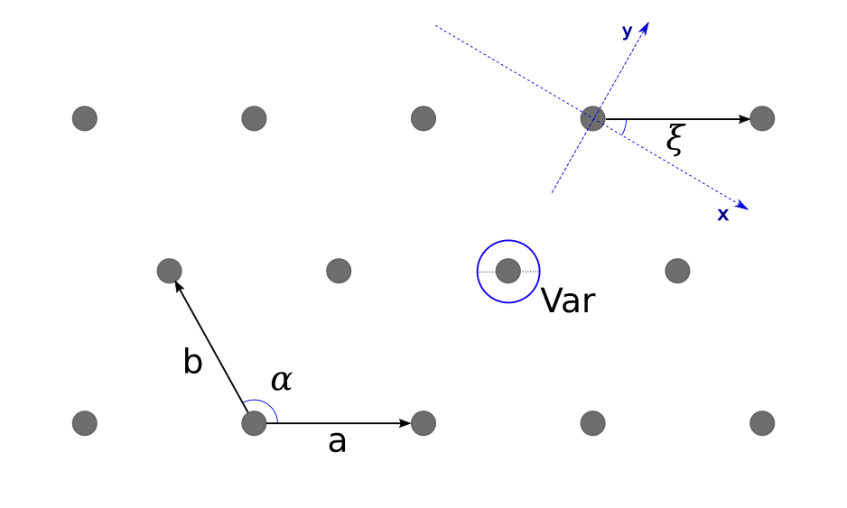
When the beam azimuthal angle $\varphi_f$ is zero, the beam direction coincides with the x-axis of the reference frame. In this case, the angle $\xi$ can be considered as the lattice rotation with respect to the beam.
Two convenience functions allow to create square and hexagonal interference functions without the need to specify the second lattice vector or the lattice angle.
# interference function of a square lattice
f = Interference2DLattice.createSquare(25.0*nm, 45.0*deg)

# interference function of a hexagonal lattice
f = Interference2DLattice.createHexagonal(25.0*nm, 45.0*deg)
Here two lattices are created, one square and one hexagonal, rotated with respect to the beam by $45^{\circ}$.
To account for finite size effects of the lattice, a decay function should be assigned to the interference function. This function encodes the loss of coherent scattering from lattice points with increasing distance between them. The origin of this loss of coherence could be attributed to the coherence lengths of the beam or to the domain structure of the lattice. The two-dimensional decay function allows for an anisotropy of this effect.
Decay functions for the one-dimensional case are explained
in the grating section.
Decay functions for two-dimensional lattices work similarly,
but require two decay_length parameters and an orientation to be defined.
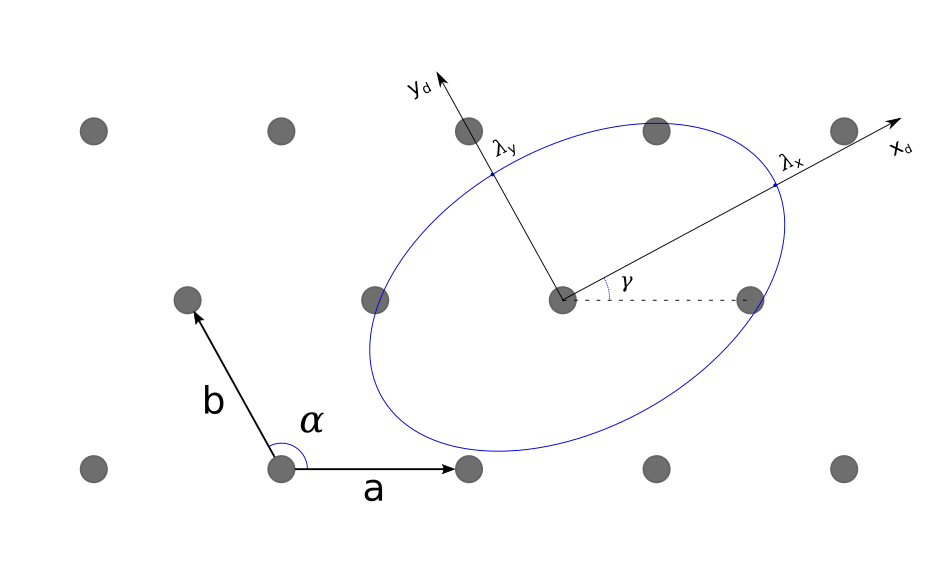
$x_d$, $y_d$ on the plot below represent an orthonormal coordinate system for the decay distribution in real space. It is rotated by the angle gamma with respect to the first lattice vector $a$. The decay lengths $\lambda_x$ and $\lambda_y$ are given in nanometers.
BornAgain supports three types of two-dimensional decay functions:
# Two-dimensional Cauchy decay function
FTDecayFunction2DCauchy(lambda_x, lambda_y, gamma=0)

# Two-dimensional Gauss decay function
FTDecayFunction2DGauss(lambda_x, lambda_y, gamma=0)

# Two-dimensional Voigt decay function
FTDecayFunction2DVoigt(lambda_x, lambda_y, eta, gamma=0)
The parameters in the Cauchy and Gauss constructors are the same:
lambda_x  : the decay length in nanometers along x-axis of the distribution
lambda_y  : the decay length in nanometers along y-axis of the distribution
gamma     : distribution orientation with respect to the first lattice vector
In the case of the Voigt distribution, an additional dimensionless parameter eta is used to balance between Gaussian and Cauchy profiles.
To set the decay function to the interference function, the setDecayFunction method should be used right after the interference function is initializated. In the code snippet below we create an interference function representing a hexagonal lattice with lattice constant 20 nm and axis vector $a$ coinciding with the beam direction. Then we set a FTDecayFunction2DCauchy decay function to it. The decay lengths are selected to be the same (1000 nm along each axis) and the $x_d$ axis of the decay function is selected to coincide with lattice vector $a$.
f = Interference2DLattice(20*nm, 20*nm, 120*deg)
f.setDecayFunction(FTDecayFunction2DCauchy(1000*nm, 1000*nm))
The computational kernel provides an automatic calculation of particle densities using the parameters of the 2D lattice. This means that the user’s setting of the particle density via the ParticleLayout.setParticleDensity() method (which is a required step in the case of a 1D interference function and radial paracrystal initialization) is ignored.
In the code below we collect together all the code required for the initialization of a two dimensional lattice interference function.
interference = ba.Interference2DLattice.createSquare(25.0*nm, 45.*deg)
pdf = ba.FTDecayFunction2DCauchy(300.0*nm, 300.0*nm)
interference.setDecayFunction(pdf)

ff = ba.Cylinder(3.*nm, 3.*nm)
cylinder = ba.Particle(m_particle, ff)
particle_layout = ba.ParticleLayout()
particle_layout.addParticle(cylinder)
particle_layout.setInterference(interference)
The complete example can be found here.