In fitting, we estimate the optimum parameters in a numerical model,
specifically a scattering simulation,
by minimizing the difference between simulated and reference data.
BornAgain supports
a variety of minimization algorithms;
choice of fitting parameters, their properties and correlations;
full control over objective function calculations, including the use of different normalizations and assignments of different masks and weights to different areas of the reference data;
possibility to fit simultaneously an arbitrary number of data sets.
In the following we will show how to fit using the BornAgain Python API.
For fitting through the graphical user interface, see GUI > Fitting.
Introductory example
In the following, a very simple example shows how to fit a parametric model to given data.
The model is a specular reflectometry scan,
with a sample consisting of 20 alternating Ti and Ni layers on a Si substrate.
Using this model, synthetic data
have been generated with GenX.
These data are part of the BornAgain sources,
testdata/specular/genx_alternating_layers.dat.gz.
To make them findable by the script,
the environment variable BA_DATA_DIR must point
to a local copy of directory testdata.
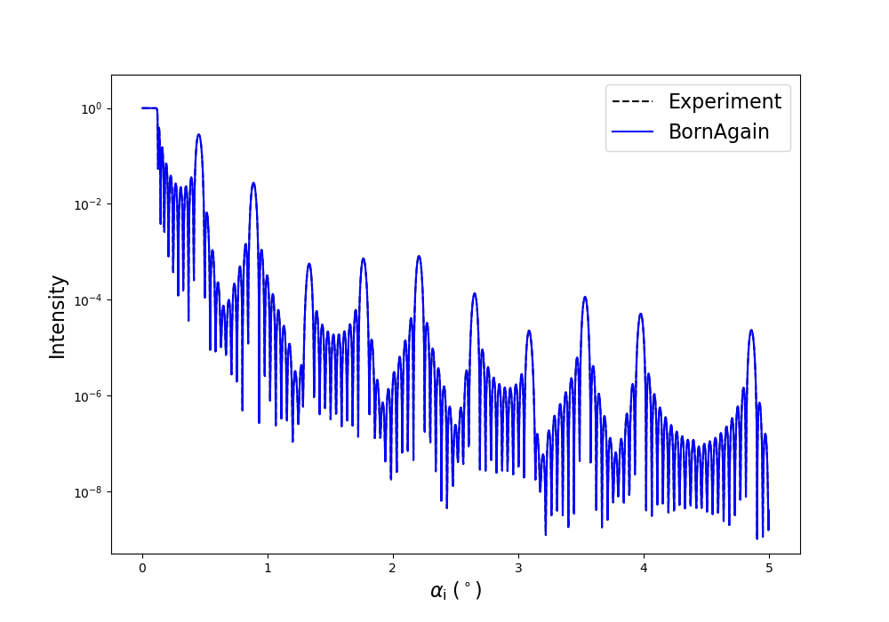
The fit model is identical to the model used for generating the data.
There is just one fit parameter, namely the thickness of the Ti layers.
The resulting fit is indistinguishable from the data:
#!/usr/bin/env python3"""
Basic example how to fit specular data.
The sample consists of twenty alternating Ti and Ni layers.
Reference data was generated with GenX.
We fit just one parameter, the thickness of the Ti layers,
which has an original value of 30 angstroms.
"""importbornagainasba,numpyasnp,osfrombornagainimportangstrom,ba_fitmonitordefload_data():datadir=os.getenv('BA_DATA_DIR','')ifnotdatadir:raiseException("Environment variable BA_DATA_DIR not set")fname=os.path.join(datadir,"specular/genx_alternating_layers.dat.gz")flags=ba.ImportSettings1D("2alpha (deg)","#","",1,2)returnba.readData1D(fname,ba.csv1D,flags)defget_sample(P):# Materialsvacuum=ba.MaterialBySLD()material_Ti=ba.MaterialBySLD("Ti",-1.9493e-06,0)material_Ni=ba.MaterialBySLD("Ni",9.4245e-06,0)material_Si=ba.MaterialBySLD("Si",2.0704e-06,0)# Layerslayer_Ti=ba.Layer(material_Ti,P["thickness_Ti"])layer_Ni=ba.Layer(material_Ni,70*angstrom)# Periodic stackn_repetitions=10stack=ba.LayerStack(n_repetitions)stack.addLayer(layer_Ti)stack.addLayer(layer_Ni)# Samplesample=ba.Sample()sample.addLayer(ba.Layer(vacuum))sample.addStack(stack)sample.addLayer(ba.Layer(material_Si))returnsampledefget_simulation(P):scan=ba.AlphaScan(data.xAxis())scan.setWavelength(1.54*angstrom)sample=get_sample(P)returnba.SpecularSimulation(scan,sample)if__name__=='__main__':data=load_data()P=ba.Parameters()P.add("thickness_Ti",50*angstrom,min=10*angstrom,max=60*angstrom)fit_objective=ba.FitObjective()fit_objective.addFitPair(get_simulation,data,1)fit_objective.initPrint(10)plot_observer=ba_fitmonitor.PlotterSpecular(pause=0.5)fit_objective.initPlot(10,plot_observer)minimizer=ba.Minimizer()result=minimizer.minimize(fit_objective.evaluate,P)fit_objective.finalize(result)plot_observer.show()
auto/Examples/fit/specular/Specular1Par.py
Explanations
The arrays (Python lists) exp_x, exp_y contain the data to be fitted.
The dictionary P contains the fit parameter.
An instance of class FitObjective defines the objective function
in terms of data $y(x)$ and fit model $f(x;P)$.
By default, it is a $\chi^2$ function, weighted with the inverse standard deviation.
The function call initPrint(10) means that values of $\chi^2$ and of all
fit parameters are printed to the terminal every 10 fit iterations.
To suppress the printing, set the function argument to 0.
Similarly, the function call initPlot(10, ...) means that
data and fit are replotted every 10 fit iterations.
In the PlotterSpecular,
the argument pause=0.5 means that after refreshing the plot the program
is put to sleep for 0.5 s.
This enables humans to observe the evolution of the plots in real time.
With pause=0, the program executes so fast that one only sees the final plot.
The actual fit is controlled by class Minimizer,
and launched by the function call minimize(...).