This is an example of a real data fit. We use our own measurements performed at the laboratory diffractometer GALAXI in Forschungszentrum Jülich.

Real-space model
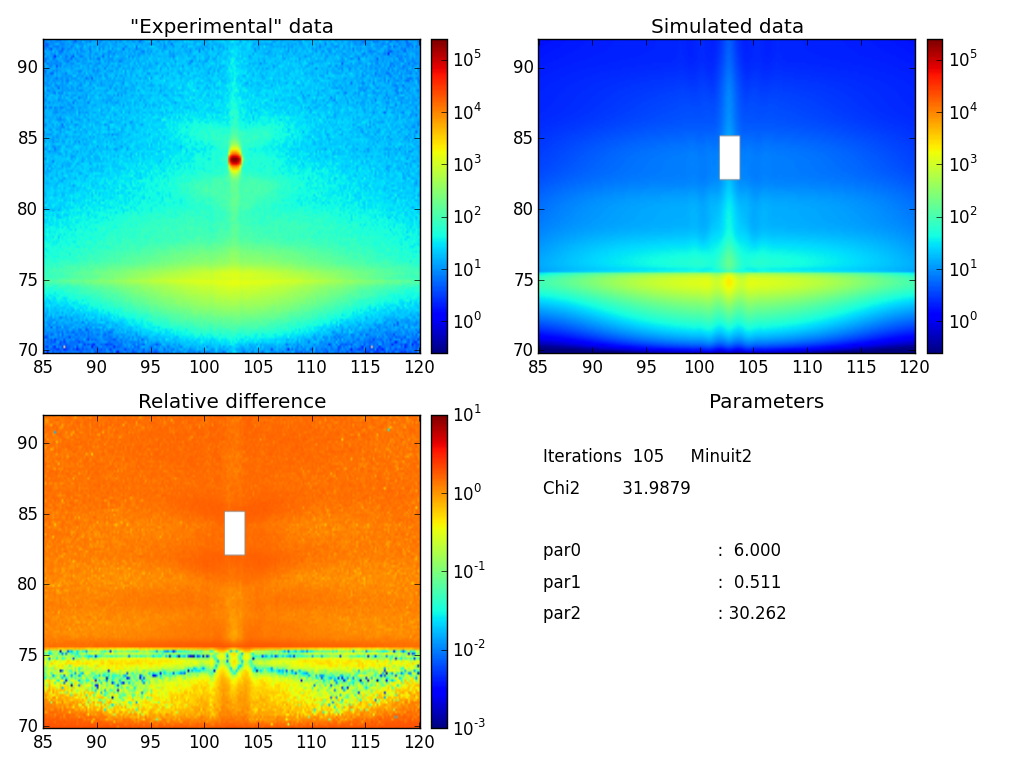
Fit window
SampleBuilder, which is able to create samples depending on parameters defined in the constructor and passed through to the create_sample method.run_fitting() function contains the initialization of the fitting kernel: loading experimental data, assignment of fit pair, fit parameters selection (line 62).To successfully simulate and fit results of some real experiment it is important to have
As an example we will use our own measurements performed at the laboratory diffractometer GALAXI in Forschungszentrum Jülich.
Our sample represents a 3-layer system (substrate, teflon and air) with Ag nanoparticles sitting on top of the teflon layer. The PILATUS 1M detector was placed at a distance of 1730 mm from the sample.
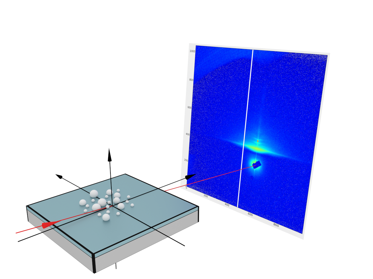
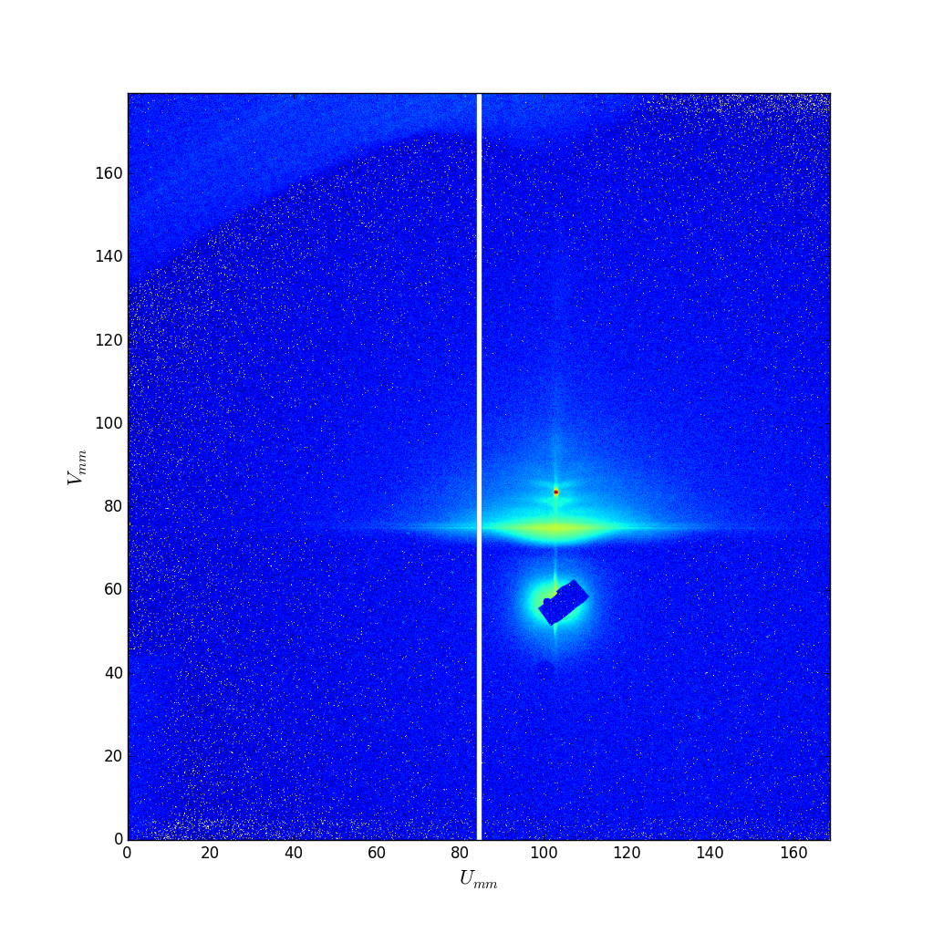
The results of the measurement are represented by the intensity image taken in certain conditions (beam wavelength, inclination angle, detector position) and stored in a 32-bit tiff file. To be able to fit these data we have to
From the experimental setup we know the following:
In BornAgain, we will represent this setup using the FlatDetector object.
First, we create a detector corresponding to a PILATUS detector by providing the number of detector bins and the detector’s size in millimeters:
npx, npy = 981, 1043
pixel_size = 0.172  # in mm
width = npx*pixel_size
height = npy*pixel_size

detector = FlatDetector(npx, width, npy, height)
Then we define the position of the direct beam in local detector coordinates (i.e. millimeters) and set the detector perpendicular to the direct beam at a certain distance:
detector_distance = 1730.0  # in mm

# position of direct beam in pixels, (0,0) corresponds to lower left corner of the image
beam_xpos, beam_ypos = 597.1, 323.4  # in pixels

# position of direct beam in local detector coordinates
u0 = beam_xpos*pixel_size  # in mm
v0 = beam_ypos*pixel_size  # in mm

detector.setPerpendicularToDirectBeam(detector_distance, u0, v0)
See also the Rectangular detector tutorial.
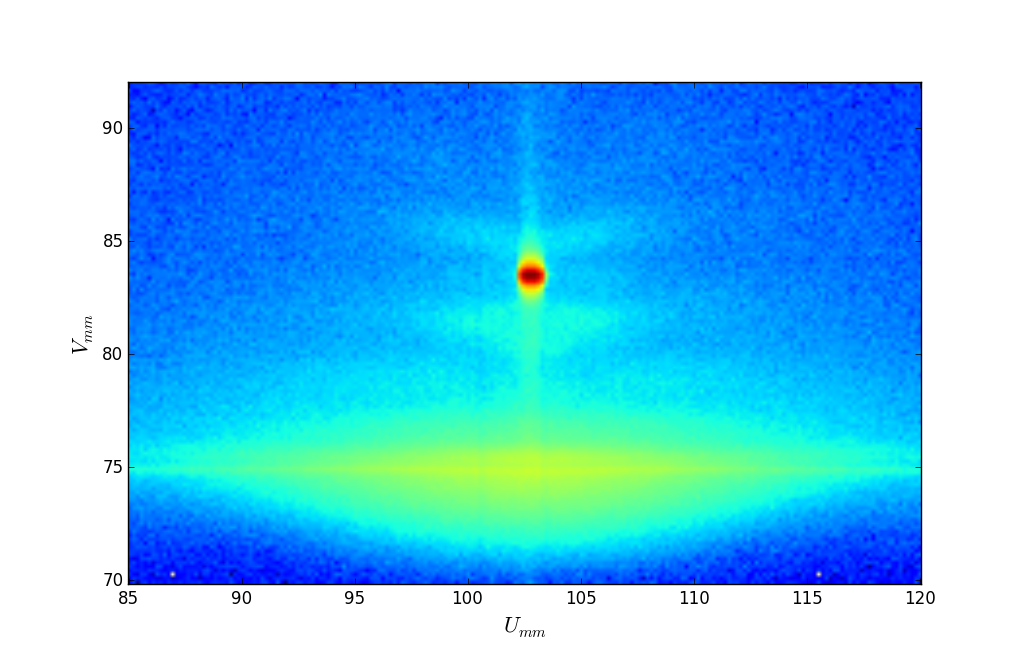
To speed-up the simulation and to avoid an influence from uninteresting areas on the fit flow it is often convenient to define a certain region of interest roi. In our example we set the roi to the rectangle with lower left corner coordinates (85.0, 70.0) and upper right corner coordinates (120.0, 92.0), where coordinates are expressed in native detector units
(mm for FlatDetector)
simulation.setRegionOfInterest(85.0, 70.0, 120.0, 92.)
The final simulation setup looks as follows:
simulation = ScatteringSimulation()
simulation.setDetector(detector)  # this is our rectangular detector
simulation.setSample(sample)  # sample creation is not covered by this tutorial
simulation.setBeamParameters(1.34*angstrom, 0.463*degree, 0.0)
simulation.setBeamIntensity(1.2e7)
simulation.setRegionOfInterest(85.0, 70.0, 120.0, 92.)
During the fit, only the part of the detector corresponding to the roi will be simulated and used for $\chi^2$ calculations.
The Fabio library provides a convenient way to import experimental data in the form of a numpy array.
import fabio

img = fabio.open("galaxi_data.tif.gz")
data = img.data.astype("float64")
The main requirement is that the shape of the numpy array coincides with the number of detector channels (i.e. npx, npy = 981, 1043 for given example).
|
|
Data to be fitted: galaxi_data.tif.gz