To add a dilute random assembly of uncorrelated particles to a layer:
layer.deposit2D(ba.Dilute2D(density, particle, ba.ParticleAlignment_BottomAligned))
layer.suspend2D(ba.Dilute2D(density, particle, ba.ParticleAlignment_TopAligned))
Argument density is the number density in nm$^{-2}$.
For argument particle, see Particle.
With deposit2D and ParticleAlignment_BottomAligned, the bottom of the particle
is placed at the layer’s bottom interface. This is appropriate for particles
sitting on a substrate. This mode must only be used for finite-thickness layers,
not for the semi-infinite bottom (substrate) or top (ambient) layer.
With suspend2D and ParticleAlignment_TopAligned, the top of the particle is
placed at the layer’s top interface. This is appropriate for particles hanging
from below an interface, such as particles embedded in a substrate just below its
top surface. This mode can be used for finite-thickness layers or the
semi-infinite bottom (substrate) layer.
For soft particles with diffuse boundaries (like FuzzySphere), use
ParticleAlignment_Centered to place the particle center at the interface.
For an incoherent mixture of different particles,
just call deposit2D multiple times with different particle structures.
To add a dense random assembly of non-overlapping but otherwise non-interacting particles to a layer:
layer.deposit2D(ba.Dense2D(density, particle, ba.ParticleAlignment_BottomAligned))
layer.suspend2D(ba.Dense2D(density, particle, ba.ParticleAlignment_TopAligned))
The scattering is computed in Percus-Yevick approximation, using the approximative structure factor of M.S. Ripoll & C.F. Tejero (1995).
Use the appropriate layer function (deposit2D or suspend2D) according to the
positioning rules described above.
In the following example, the sample is a dense random assembly of disks on a substrate. GISAS has been simulated (a) assuming that the disks are completely uncorrelated, as in an ideal gas, and (b) taking into account that the disks cannot overlap, using the hard-disk liquid model. The figure shows horizontal cuts through these GISAS patterns.
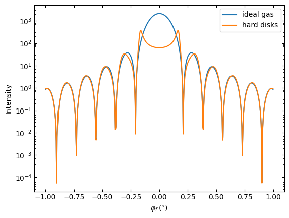
GISAS intensity at $\alpha_f=0.8^\circ$
|
|