Disordered 3D particle assemblies

Class Disordered3D models random assemblies of uncorrelated particles in the bulk. It can be used for thin films as long as the film thickness is substantially greater than the particle diameter.

Possible applications are

  • nanoparticle-filled polymer films,
  • colloidal suspensions, and
  • any other system where particles (or holes) are dispersed in a matrix.

Creating a 3D assembly

To fill a layer with randomly distributed particles, use the function Layer.plugLiquid:

layer = ba.Layer(matrix_material, thickness)
layer.plugLiquid(density, particle[, approximation_flag])

If the layer contains an incoherent mixture of the disordered assembly and something else, then a Disordered3D object must be explicitly created, and added to the layer with a Layer.addStruct function call:

layer = ba.Layer(matrix_material, thickness)
disordered = ba.Disordered3D(density, particle[, approximation_flag])
layer.addStruct(weight, disordered)

Parameters:

  • density: Volume number density in nm⁻³ (particles per cubic nanometer)
  • particle: The particle to distribute throughout the layer
  • approximation_flag (optional): see below, Correlation models
  • weight (second form only): incoherent weight, between 0 and 1

Correlation models

For dilute systems, particles scatter independently. For denser systems, spatial correlations between particles affect the scattering. Two models are available:

# Dilute approximation (default): no correlations
layer.plugLiquid(density, particle, ba.Random3D_Dilute)

# Percus-Yevick hard-sphere model: accounts for excluded volume
layer.plugLiquid(density, particle, ba.Random3D_PY)

The Percus-Yevick approximation models hard-sphere correlations and becomes important when the particle volume fraction is significant.

Requirements

3D assemblies require material averaging to be enabled (the default). The layer thickness must be finite and larger than the particle size.

Examples

Dilute film

Spherical nanoparticles dispersed in a substrate layer:

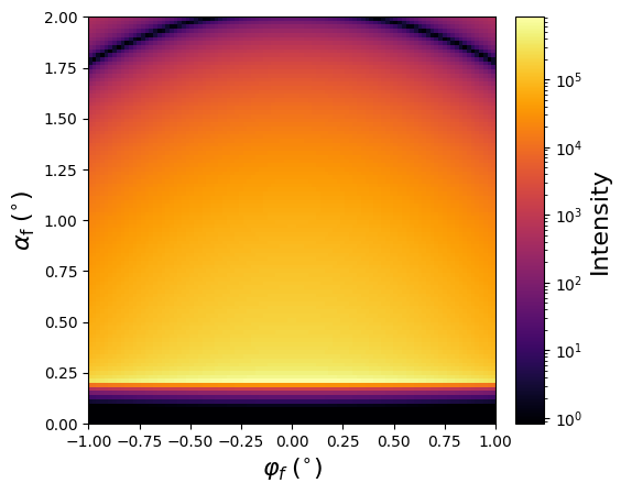
Scattering from dilute film

 1
 2
 3
 4
 5
 6
 7
 8
 9
10
11
12
13
14
15
16
17
18
19
20
21
22
23
24
25
26
27
28
29
30
31
32
33
34
35
36
37
38
39
40
41
42
43
44
45
46
47
#!/usr/bin/env python3
"""
Dilute film of small spheres
"""
import bornagain as ba
from bornagain import ba_plot as bp, deg, nm, nm3


def get_sample():
    # Materials
    material_particle = ba.RefractiveMaterial("Particle", 0.0006, 2e-08)
    material_substrate = ba.RefractiveMaterial("Substrate", 6e-06, 2e-08)
    vacuum = ba.Vacuum()

    # Particles
    ff = ba.Sphere(2*nm)
    particle = ba.Particle(material_particle, ff)

    # Layers
    layer_1 = ba.Layer(vacuum)
    layer_2 = ba.Layer(material_substrate, 30*nm)
    layer_3 = ba.Layer(material_substrate)
    layer_2.plugLiquid(.0005/nm3, particle)

    # Sample
    sample = ba.Sample()
    sample.addLayer(layer_1)
    sample.addLayer(layer_2)
    sample.addLayer(layer_3)

    return sample


def get_simulation(sample):
    beam = ba.Beam(1e9, 0.1*nm, 0.2*deg)
    n = 100
    detector = ba.SphericalDetector(n, -1*deg, 1*deg, n, 0., 2*deg)
    simulation = ba.ScatteringSimulation(beam, sample, detector)
    return simulation


if __name__ == '__main__':
    sample = get_sample()
    simulation = get_simulation(sample)
    result = simulation.simulate()
    bp.plot_datafield(result)
    bp.plt.show()
auto/Examples/scatter2d/DiluteFilm.py

Dense film: dilute vs Percus-Yevick

Comparison of dilute approximation and Percus-Yevick model for a denser film. The PY model shows structure factor oscillations due to hard-sphere correlations:

Dilute vs Percus-Yevick

scatter2d/DenseFilm.py
 1
 2
 3
 4
 5
 6
 7
 8
 9
10
11
12
13
14
15
16
17
18
19
20
21
22
23
24
25
26
27
28
29
30
31
32
33
34
35
36
37
38
39
40
41
42
43
44
45
46
47
48
49
50
51
52
#!/usr/bin/env python3
"""
Dilute film of small spheres
"""
import bornagain as ba
from bornagain import ba_plot as bp, deg, nm, nm3


def get_sample(approximation):
    # Materials
    material_particle = ba.RefractiveMaterial("Particle", 0.0006, 2e-08)
    material_substrate = ba.RefractiveMaterial("Substrate", 6e-06, 2e-08)
    vacuum = ba.Vacuum()

    # Particles
    ff = ba.Sphere(4*nm)
    particle = ba.Particle(material_particle, ff)

    # Layers
    layer_1 = ba.Layer(vacuum)
    layer_2 = ba.Layer(material_substrate, 30*nm)
    layer_3 = ba.Layer(material_substrate)
    layer_2.plugLiquid(.002/nm3, particle, approximation)

    # Sample
    sample = ba.Sample()
    sample.addLayer(layer_1)
    sample.addLayer(layer_2)
    sample.addLayer(layer_3)

    return sample


def get_simulation(sample):
    beam = ba.Beam(1e9, 0.1*nm, 0.2*deg)
    n = 100
    # Just compute a 1d cut at phi=0
    detector = ba.SphericalDetector(1, -1*deg, 1*deg, n, 0., 2*deg)
    simulation = ba.ScatteringSimulation(beam, sample, detector)
    return simulation


if __name__ == '__main__':
    samples = [
        get_sample(ba.Random3D_Dilute),
        get_sample(ba.Random3D_PY)
    ]
    results = [ get_simulation(sample).simulate() for sample in samples ]
    for r in results:
        bp.plot_datafield(r)
    bp.plt.legend(['Dilute', 'Percus-Yevick'])
    bp.plt.show()
auto/Examples/scatter2d/DenseFilm.py

Film vs monolayer

Comparison between a 3D film (plugLiquid) and a 2D monolayer (depositParticle). As film thickness increases, the scattering pattern evolves from the monolayer limit:

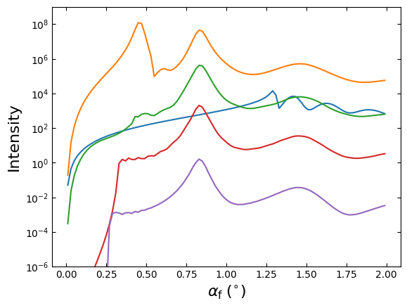
Film thickness dependence

scatter2d/FilmVsMonolayer.py
auto/Examples/scatter2d/FilmVsMonolayer.py